Table of Content

• 1 Introduction
• 2 Presentation of the data records used
• 3 Dividing the data into a training part and a test part
• 4 Removing problematic features
• 4.1 Machine dataset
• 4.2 Cars dataset
• 5 Assessing linear regression models
• 6 How to check some summary outputs individually
• 6.1 Residual analysis
• 6.2 Significance tests for linear regression
• 6.3 Residual standard error (RSE)
• 6.4 R²
• 7 Test set performance with the MSE
• 8 Problems with linear regression
• 8.1 Multicollinearity
• 8.2 Outliers
• 8.2.1 Compare RSE
• 8.2.2 Compare MSE
• 9 Future selection
• 9.1 Forward selection
• 9.2 Backward selection
• 9.3 Comparing the calculated MSE
• 10 Regularization
• 11 Conclusion

1 Introduction

I have already written several general contributions on linear regression models (“here” and “here”). Likewise, I have already taken up the issue of how linear regression models can be trained and tested (“Machine Learning - Training and Testing Sets: Regression Modeling”) and how unimportant variables can be identified (“Machine Learning - Regression Regularization”).

In this publication, the prediction of the dependent variables from two different data networks should be central. In particular, the potential for improvement of the predictive power of the created models shall be considered.

For this post the dataset machine from the UCI- Machine Learning Repository platform “UCI” was used as well as the dataset cars from the caret-package. A copy of the records is available at https://drive.google.com/open?id=1tMtpU5xEkijF-GceVEmGwRQCVrhWNrvf (machine) and https://drive.google.com/open?id=1E_NWwWEBBby456SuHt3qxHrsDpTzcUuv (cars).

2 Presentation of the data records used

The first dataframe (machine) contains the characteristics of different CPU models, such as the cycle time and the amount cache memory. PRP will be the dependent variable.The variables that are superfluous for this study are excluded in advance.

machine <- machine[, 4:10]
head(machine, n = 5)

## # A tibble: 5 x 7
##    MYCT  MMIN  MMAX  CACH CHMIN CHMAX   PRP
##   <int> <int> <int> <int> <int> <int> <int>
## 1   125   256  6000   256    16   128   198
## 2    29  8000 32000    32     8    32   269
## 3    29  8000 32000    32     8    32   220
## 4    29  8000 32000    32     8    32   172
## 5    29  8000 16000    32     8    16   132

The second datafame (cars) contains details about different used car components, such as the number of cylinders or the number of miles the car has been driven.

cars <- cars[, -1]
glimpse(cars)

## Observations: 804
## Variables: 18
## $ Price       <dbl> 22661.05, 21725.01, 29142.71, 30731.94, 33358.77, ...
## $ Mileage     <int> 20105, 13457, 31655, 22479, 17590, 23635, 17381, 2...
## $ Cylinder    <int> 6, 6, 4, 4, 4, 4, 4, 4, 4, 4, 4, 4, 4, 4, 4, 4, 4,...
## $ Doors       <int> 4, 2, 2, 2, 2, 2, 2, 2, 2, 4, 4, 4, 4, 4, 4, 4, 4,...
## $ Cruise      <int> 1, 1, 1, 1, 1, 1, 1, 1, 1, 1, 1, 1, 1, 1, 1, 1, 1,...
## $ Sound       <int> 0, 1, 1, 0, 1, 0, 1, 0, 0, 0, 1, 1, 1, 0, 1, 0, 1,...
## $ Leather     <int> 0, 0, 1, 0, 1, 0, 1, 1, 0, 1, 0, 1, 1, 0, 1, 1, 1,...
## $ Buick       <int> 1, 0, 0, 0, 0, 0, 0, 0, 0, 0, 0, 0, 0, 0, 0, 0, 0,...
## $ Cadillac    <int> 0, 0, 0, 0, 0, 0, 0, 0, 0, 0, 0, 0, 0, 0, 0, 0, 0,...
## $ Chevy       <int> 0, 1, 0, 0, 0, 0, 0, 0, 0, 0, 0, 0, 0, 0, 0, 0, 0,...
## $ Pontiac     <int> 0, 0, 0, 0, 0, 0, 0, 0, 0, 0, 0, 0, 0, 0, 0, 0, 0,...
## $ Saab        <int> 0, 0, 1, 1, 1, 1, 1, 1, 1, 1, 1, 1, 1, 1, 1, 1, 1,...
## $ Saturn      <int> 0, 0, 0, 0, 0, 0, 0, 0, 0, 0, 0, 0, 0, 0, 0, 0, 0,...
## $ convertible <int> 0, 0, 1, 1, 1, 1, 1, 1, 1, 0, 0, 0, 0, 0, 0, 0, 0,...
## $ coupe       <int> 0, 1, 0, 0, 0, 0, 0, 0, 0, 0, 0, 0, 0, 0, 0, 0, 0,...
## $ hatchback   <int> 0, 0, 0, 0, 0, 0, 0, 0, 0, 0, 0, 0, 0, 0, 0, 0, 0,...
## $ sedan       <int> 1, 0, 0, 0, 0, 0, 0, 0, 0, 1, 1, 1, 1, 1, 1, 1, 1,...
## $ wagon       <int> 0, 0, 0, 0, 0, 0, 0, 0, 0, 0, 0, 0, 0, 0, 0, 0, 0,...

3 Dividing the data into a training part and a test part

set.seed(223356)
machine_sampling_vector <- createDataPartition(machine$PRP, p = 0.85, list = FALSE)
machine_train <- machine[machine_sampling_vector,]
machine_train_labels <- machine$PRP[machine_sampling_vector]
machine_test <- machine[-machine_sampling_vector,]
machine_test_labels <- machine$PRP[-machine_sampling_vector]
machine_train_features <- machine[, 1:6]

cars_sampling_vector <- createDataPartition(cars$Price, p = 0.85, list = FALSE)
cars_train <- cars[cars_sampling_vector,]
cars_train_labels <- cars$Price[cars_sampling_vector]
cars_test <- cars[-cars_sampling_vector,]
cars_test_labels <- cars$Price[-cars_sampling_vector]
cars_train_features <- cars[,-1]

4 Removing problematic features

Highly correlated variables can influence the prediction of a linear model. From this point of view, it is recommended to overcome this in the first step and to exclude problematic features.

4.1 Machine dataset

machine_correlations <- cor(machine_train_features)
findCorrelation(machine_correlations)

## integer(0)

As we can see, there is no correlation above 0.9 (by default). Let’s check correlations of 0.75 by this.

findCorrelation(machine_correlations, cutoff = 0.75)

## [1] 3

cor(machine_train$MMIN, machine_train$MMAX)

## [1] 0.7434639

Ok we have three of them but 0.75 should not be problematic.

findLinearCombos(machine_correlations)

## $linearCombos
## list()
## 
## $remove
## NULL

4.2 Cars dataset

Let’s have a look at the cars dataset.

cars_cor <- cor(cars_train_features)
findCorrelation(cars_cor)

## integer(0)

findCorrelation(cars_cor, cutoff = 0.75)

## [1] 3

Again three correlations between 0.75 and 0.9 (by default). One example of these three are the correlation betwenn the variables Doors and Coupe.

cor(cars$Doors,cars$coupe)

## [1] -0.8254435

table(cars$coupe,cars$Doors)

##    
##       2   4
##   0  50 614
##   1 140   0

Another usefull function is the findLinearCombos function to detect exact linear combinations of other features.

findLinearCombos(cars)

## $linearCombos
## $linearCombos[[1]]
## [1] 15  4  8  9 10 11 12 13 14
## 
## $linearCombos[[2]]
##  [1] 18  4  8  9 10 11 12 13 16 17
## 
## 
## $remove
## [1] 15 18

Here we are advised to drop the coupe and wagon columns, which are the 15th and 18th features, respectively, because they are exact linear combinations of other features. Note that the division into a training part and a test part must be redone.

set.seed(323356)
cars <- cars[,c(-15, -18)]
cars_sampling_vector <- createDataPartition(cars$Price, p = 0.85, list = FALSE)
cars_train <- cars[cars_sampling_vector,]
cars_train_labels <- cars$Price[cars_sampling_vector]
cars_test <- cars[-cars_sampling_vector,]
cars_test_labels <- cars$Price[-cars_sampling_vector]
cars_train_features <- cars[,-1]

5 Assessing linear regression models

Once all the problematic features have been identified and excluded, it is time to create the regression models.

machine_model1 <- lm(PRP ~ ., data = machine_train)
cars_model1 <- lm(Price ~ ., data = cars_train)

Here the summary for the machine_model1:

summary(machine_model1)

## 
## Call:
## lm(formula = PRP ~ ., data = machine_train)
## 
## Residuals:
##     Min      1Q  Median      3Q     Max 
## -195.49  -27.38    5.26   24.94  371.14 
## 
## Coefficients:
##               Estimate Std. Error t value Pr(>|t|)    
## (Intercept) -5.012e+01  8.764e+00  -5.719 4.66e-08 ***
## MYCT         3.940e-02  1.843e-02   2.138   0.0339 *  
## MMIN         1.085e-02  2.166e-03   5.012 1.33e-06 ***
## MMAX         6.580e-03  7.103e-04   9.263  < 2e-16 ***
## CACH         7.068e-01  1.446e-01   4.889 2.32e-06 ***
## CHMIN       -7.129e-01  8.873e-01  -0.803   0.4228    
## CHMAX        1.352e+00  2.317e-01   5.835 2.61e-08 ***
## ---
## Signif. codes:  0 '***' 0.001 '**' 0.01 '*' 0.05 '.' 0.1 ' ' 1
## 
## Residual standard error: 59.49 on 172 degrees of freedom
## Multiple R-squared:  0.8512, Adjusted R-squared:  0.846 
## F-statistic:   164 on 6 and 172 DF,  p-value: < 2.2e-16

And here the summary for the cars_model1:

summary(cars_model1)

## 
## Call:
## lm(formula = Price ~ ., data = cars_train)
## 
## Residuals:
##     Min      1Q  Median      3Q     Max 
## -9926.1 -1527.6   165.4  1505.8 12932.1 
## 
## Coefficients: (1 not defined because of singularities)
##               Estimate Std. Error t value Pr(>|t|)    
## (Intercept) -1.150e+03  1.103e+03  -1.042  0.29760    
## Mileage     -1.865e-01  1.385e-02 -13.471  < 2e-16 ***
## Cylinder     3.742e+03  1.240e+02  30.187  < 2e-16 ***
## Doors        1.542e+03  2.853e+02   5.405 9.04e-08 ***
## Cruise       3.251e+02  3.295e+02   0.987  0.32423    
## Sound        4.053e+02  2.601e+02   1.558  0.11967    
## Leather      7.858e+02  2.769e+02   2.838  0.00467 ** 
## Buick        6.691e+02  6.234e+02   1.073  0.28350    
## Cadillac     1.342e+04  7.002e+02  19.159  < 2e-16 ***
## Chevy       -7.211e+02  4.952e+02  -1.456  0.14575    
## Pontiac     -1.572e+03  5.475e+02  -2.871  0.00421 ** 
## Saab         1.221e+04  6.268e+02  19.474  < 2e-16 ***
## Saturn              NA         NA      NA       NA    
## convertible  1.113e+04  5.975e+02  18.623  < 2e-16 ***
## hatchback   -6.393e+03  6.892e+02  -9.276  < 2e-16 ***
## sedan       -4.516e+03  4.903e+02  -9.211  < 2e-16 ***
## ---
## Signif. codes:  0 '***' 0.001 '**' 0.01 '*' 0.05 '.' 0.1 ' ' 1
## 
## Residual standard error: 2968 on 669 degrees of freedom
## Multiple R-squared:  0.9151, Adjusted R-squared:  0.9133 
## F-statistic: 515.2 on 14 and 669 DF,  p-value: < 2.2e-16

Please note the following message from the output: “Coefficients: (1 not defined because of singularities)”. This occurs because we still have features whose effect on the output is indiscernible form other features due to underlying dependencies. We can identify this variable using the alias function.

alias(cars_model1)

## Model :
## Price ~ Mileage + Cylinder + Doors + Cruise + Sound + Leather + 
##     Buick + Cadillac + Chevy + Pontiac + Saab + Saturn + convertible + 
##     hatchback + sedan
## 
## Complete :
##        (Intercept) Mileage Cylinder Doors Cruise Sound Leather Buick
## Saturn  1           0       0        0     0      0     0      -1   
##        Cadillac Chevy Pontiac Saab convertible hatchback sedan
## Saturn -1       -1    -1      -1    0           0         0

Now we know, that we have to remove the Saturn variable.

cars_model2 <- lm(Price ~. -Saturn, data = cars_train)
summary(cars_model2)

## 
## Call:
## lm(formula = Price ~ . - Saturn, data = cars_train)
## 
## Residuals:
##     Min      1Q  Median      3Q     Max 
## -9926.1 -1527.6   165.4  1505.8 12932.1 
## 
## Coefficients:
##               Estimate Std. Error t value Pr(>|t|)    
## (Intercept) -1.150e+03  1.103e+03  -1.042  0.29760    
## Mileage     -1.865e-01  1.385e-02 -13.471  < 2e-16 ***
## Cylinder     3.742e+03  1.240e+02  30.187  < 2e-16 ***
## Doors        1.542e+03  2.853e+02   5.405 9.04e-08 ***
## Cruise       3.251e+02  3.295e+02   0.987  0.32423    
## Sound        4.053e+02  2.601e+02   1.558  0.11967    
## Leather      7.858e+02  2.769e+02   2.838  0.00467 ** 
## Buick        6.691e+02  6.234e+02   1.073  0.28350    
## Cadillac     1.342e+04  7.002e+02  19.159  < 2e-16 ***
## Chevy       -7.211e+02  4.952e+02  -1.456  0.14575    
## Pontiac     -1.572e+03  5.475e+02  -2.871  0.00421 ** 
## Saab         1.221e+04  6.268e+02  19.474  < 2e-16 ***
## convertible  1.113e+04  5.975e+02  18.623  < 2e-16 ***
## hatchback   -6.393e+03  6.892e+02  -9.276  < 2e-16 ***
## sedan       -4.516e+03  4.903e+02  -9.211  < 2e-16 ***
## ---
## Signif. codes:  0 '***' 0.001 '**' 0.01 '*' 0.05 '.' 0.1 ' ' 1
## 
## Residual standard error: 2968 on 669 degrees of freedom
## Multiple R-squared:  0.9151, Adjusted R-squared:  0.9133 
## F-statistic: 515.2 on 14 and 669 DF,  p-value: < 2.2e-16

Perfect!

6 How to check some summary outputs individually

All the information which we receive with the summary command can also be calculated automatically:

6.1 Residual analysis

A residual is simply the error our model makes for a paritcular observation.

summary(cars_model2$residuals)

##    Min. 1st Qu.  Median    Mean 3rd Qu.    Max. 
## -9926.1 -1527.6   165.4     0.0  1505.8 12932.1

mean(cars_train$Price)

## [1] 21421.88

With this information we can say that the average selling price of a car in our training data is around 21k Dollar, and 50% of our predictions are roughly within +- 1.6k of the correct value.

A useful way to graphically compare the quantiles of the distributions of two quantitative variables is the quantile-quantile diagram.

par(mfrow = c(2, 1))
machine_residuals <- machine_model1$residuals
qqnorm(machine_residuals, main = "Normal Q-Q Plot for CPU data set")
qqline(machine_residuals)
cars_residuals <- cars_model2$residuals
qqnorm(cars_residuals, main = "Normal Q-Q Plot for Cars data set")
qqline(cars_residuals)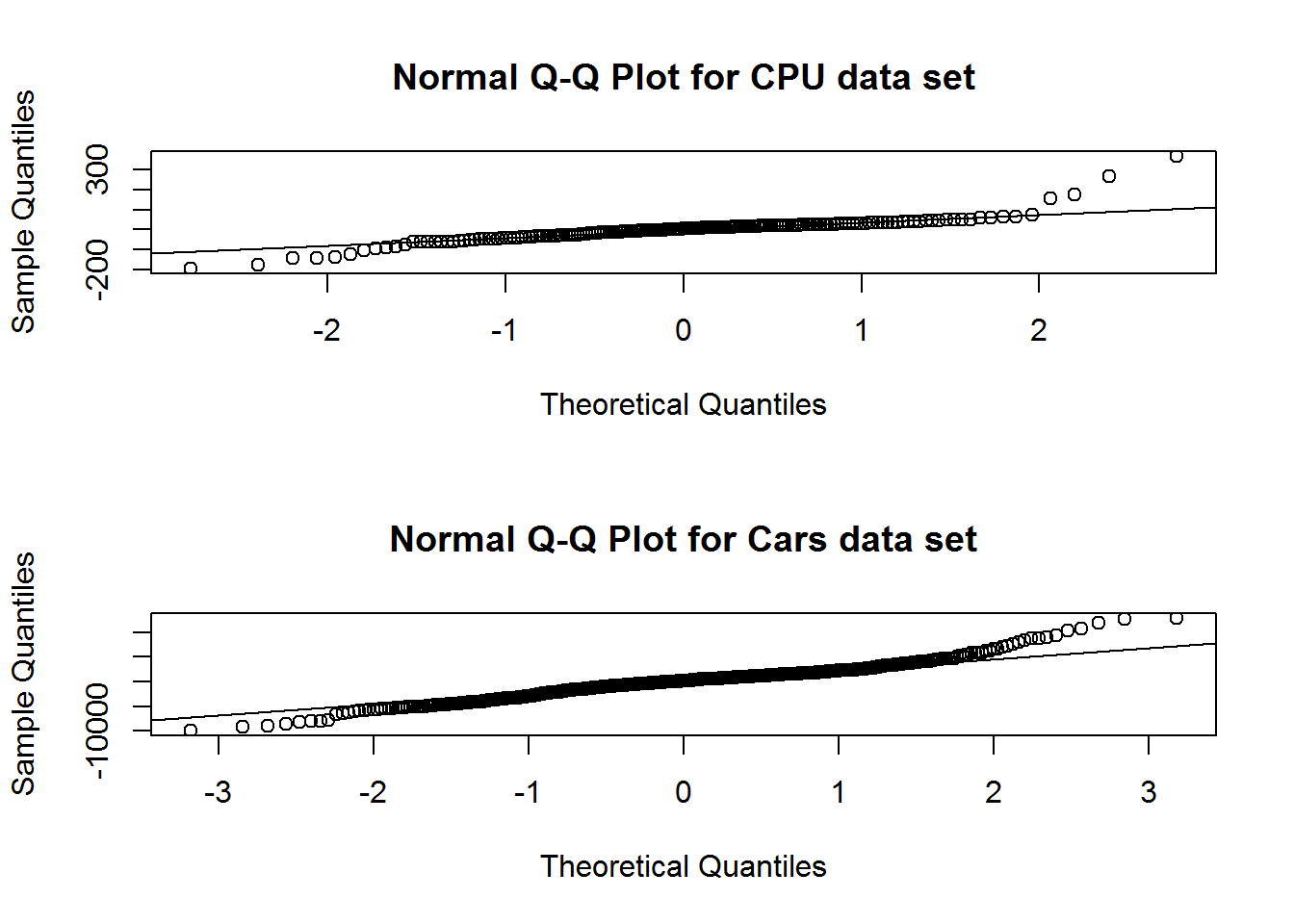

As we can see the residuals from both models seem to lie reasonably close to the theoretical quantiles of a normal distribution, although the fit isn’t perfect, as is typical with most real-world data.

6.2 Significance tests for linear regression

Let’s have a look at the machine_model1 output again:

summary(machine_model1)

## 
## Call:
## lm(formula = PRP ~ ., data = machine_train)
## 
## Residuals:
##     Min      1Q  Median      3Q     Max 
## -195.49  -27.38    5.26   24.94  371.14 
## 
## Coefficients:
##               Estimate Std. Error t value Pr(>|t|)    
## (Intercept) -5.012e+01  8.764e+00  -5.719 4.66e-08 ***
## MYCT         3.940e-02  1.843e-02   2.138   0.0339 *  
## MMIN         1.085e-02  2.166e-03   5.012 1.33e-06 ***
## MMAX         6.580e-03  7.103e-04   9.263  < 2e-16 ***
## CACH         7.068e-01  1.446e-01   4.889 2.32e-06 ***
## CHMIN       -7.129e-01  8.873e-01  -0.803   0.4228    
## CHMAX        1.352e+00  2.317e-01   5.835 2.61e-08 ***
## ---
## Signif. codes:  0 '***' 0.001 '**' 0.01 '*' 0.05 '.' 0.1 ' ' 1
## 
## Residual standard error: 59.49 on 172 degrees of freedom
## Multiple R-squared:  0.8512, Adjusted R-squared:  0.846 
## F-statistic:   164 on 6 and 172 DF,  p-value: < 2.2e-16

We can compute some figures manually, eg. the t-value and p-value of the MYCT variable:

q <- 3.940e-02 / 1.843e-02
q

## [1] 2.137819

pt(q, df = 172, lower.tail = F) * 2

## [1] 0.03394365

6.3 Residual Standard Error (RSE)

We define a metric known as the Residual Standard Error, which estimates the standard deviation of our model compared to the target function.

We can compute the RSE for our two models using the preceding formular as follows:

n_machine <- nrow(machine_train)
k_machine <- length(machine_model1$coefficients) - 1
sqrt(sum(machine_model1$residuals ^ 2) / (n_machine - k_machine - 1))

## [1] 59.48601

n_cars <- nrow(cars_train)
k_cars <- length(cars_model2$coefficients) - 1
sqrt(sum(cars_model2$residuals ^ 2) / (n_cars - k_cars - 1))

## [1] 2968.038

To interpret the RSE values for our two models, we neet to compare them with the mean of our output variables.

mean(machine_train$PRP)

## [1] 104.3799

mean(cars_train$Price)

## [1] 21421.88

6.4 R²

Now let’s compute R² manually to compare different regression models.

compute_rsquared <- function(x, y) {
  rss <- sum((x - y) ^ 2)
  tss <- sum((y - mean(y)) ^ 2)
  return(1 - (rss / tss))
}

compute_rsquared(machine_model1$fitted.values, machine_train$PRP)

## [1] 0.8512293

compute_rsquared(cars_model2$fitted.values, cars_train$Price)

## [1] 0.915124

6.5 Adjusted R²

We can also do the same manual calculation for the adjusted R².

compute_adjusted_rsquared <- function(x, y, k) {
  n <- length(y)
  r2 <- compute_rsquared(x, y)
  return(1 - ((1 - r2) * (n - 1) / (n - k - 1)))
}

compute_adjusted_rsquared(machine_model1$fitted.values, machine_train$PRP, k_machine)

## [1] 0.8460396

compute_adjusted_rsquared(cars_model2$fitted.values, cars_train$Price, k_cars)

## [1] 0.9133479

7 Test set performance with the MSE

Now it’s time to check the test set performance of our models. We can do this by the Mean Squared Error (MSE).

machine_model1_predictions <- predict(machine_model1, machine_test)
cars_model2_predictions <- predict(cars_model2, cars_test)

Here is the required function for it:

compute_mse <- function(predictions, actual) { 
  mean( (predictions - actual) ^ 2 ) 
}

7.1 MSE for the machine dataset

Now we can compare the training and the test MSE for both models

compute_mse(machine_model1$fitted.values, machine_train$PRP)

## [1] 3400.205

compute_mse(machine_model1_predictions, machine_test$PRP)

## [1] 4851.117

7.2 MSE for the cars dataset

compute_mse(cars_model2$fitted.values, cars_train$Price)

## [1] 8616064

compute_mse(cars_model2_predictions, cars_test$Price)

## [1] 6642865

8 Problems with linear regression

In my post “Regression Analysis” paragraph 5 Model assumption I have already addressed several aspects that must be taken into account when creating a regression model. For the present investigation of the two datasets two aspects are dealt with in detail.

8.1 Multicollinearity

Multicollinearity is a problem of regression analysis and occurs when two or more explanatory variables have a very strong correlation with each other. We can check this with the vif function.

vif(cars_model2)

##     Mileage    Cylinder       Doors      Cruise       Sound     Leather 
##    1.014590    2.305431    4.627138    1.556113    1.132148    1.190324 
##       Buick    Cadillac       Chevy     Pontiac        Saab convertible 
##    2.701517    3.408751    4.548446    3.666666    3.648418    1.633317 
##   hatchback       sedan 
##    2.266794    4.429628

These values can also be calculated manually by us. Here is the example for the calculation of the value for the variable Sedan

sedan_model <- lm(sedan ~ .-Price -Saturn, data = cars_train)
sedan_r2 <- compute_rsquared(sedan_model$fitted.values, cars_train$sedan)
1 / (1-sedan_r2)

## [1] 4.429628

8.2 Outliers

Outliers should always be taken into account in predictive models, as they can greatly influence the forecast, as the following example shows:

scatterplot(machine_model1$fitted.values, machine_model1$residuals, id = TRUE, xlab = "Fitted Values", ylab = "Residuals", main = "Searching for outliers")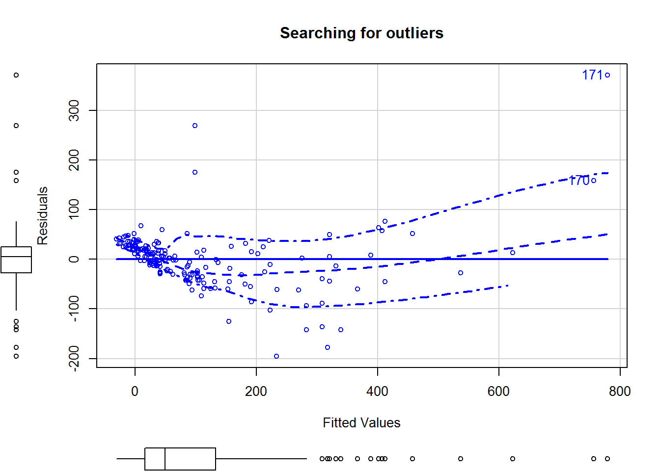

## [1] 170 171

As we can see in the graphic line 171 is an outlier. Now we check what effect it has when we exclude line 171 from the training part.

machine_model2 <- lm(PRP ~ ., data = machine_train[!(rownames(machine_train)) %in% c(171),])

summary(machine_model2)

## 
## Call:
## lm(formula = PRP ~ ., data = machine_train[!(rownames(machine_train)) %in% 
##     c(171), ])
## 
## Residuals:
##      Min       1Q   Median       3Q      Max 
## -168.193  -21.945    2.989   19.127  301.877 
## 
## Coefficients:
##               Estimate Std. Error t value Pr(>|t|)    
## (Intercept) -3.558e+01  7.461e+00  -4.769 3.95e-06 ***
## MYCT         2.766e-02  1.536e-02   1.801 0.073509 .  
## MMIN         1.241e-02  1.807e-03   6.866 1.17e-10 ***
## MMAX         5.302e-03  6.072e-04   8.732 2.21e-15 ***
## CACH         6.656e-01  1.201e-01   5.539 1.13e-07 ***
## CHMIN        9.020e-01  7.591e-01   1.188 0.236328    
## CHMAX        7.646e-01  2.035e-01   3.756 0.000236 ***
## ---
## Signif. codes:  0 '***' 0.001 '**' 0.01 '*' 0.05 '.' 0.1 ' ' 1
## 
## Residual standard error: 49.4 on 171 degrees of freedom
## Multiple R-squared:  0.8605, Adjusted R-squared:  0.8556 
## F-statistic: 175.8 on 6 and 171 DF,  p-value: < 2.2e-16

8.2.1 Compare RSE

sqrt(sum(machine_model1$residuals ^ 2) / (n_machine - k_machine - 1))

## [1] 59.48601

k_machine <- length(machine_model2$coefficients) - 1
sqrt(sum(machine_model2$residuals ^ 2) / (n_machine - k_machine - 1))

## [1] 49.25533

8.2.2 Compare MSE

compute_mse(machine_model1_predictions, machine_test$PRP)

## [1] 4851.117

machine_model2_predictions <- predict(machine_model2, machine_test)
compute_mse(machine_model2_predictions, machine_test$PRP)

## [1] 4426.187

9 Future selection

Future selection is a machine learning approach, that uses only a subset of the available features for a learning algorithm. To do this we need the null-modell of both regression models.

machine_model_null <- lm(PRP ~ 1, data = machine_train[!(rownames(machine_train)) %in% c(171),])
cars_model_null <- lm(Price ~ 1, data = cars_train)

There are two types of future selection to operate: the forward selection and the backward selection (both demonstrated below). Note that the lower the AIC, the better the model.

9.1 Forward selection

machine_model3 <- step(machine_model_null, scope = list(lower = machine_model_null, upper = machine_model2), direction = "forward")

## Start:  AIC=1733.86
## PRP ~ 1
## 
##         Df Sum of Sq     RSS    AIC
## + MMAX   1   2198118  793525 1499.6
## + MMIN   1   1895917 1095725 1557.1
## + CACH   1   1304264 1687379 1633.9
## + CHMIN  1   1073780 1917862 1656.7
## + CHMAX  1    830598 2161045 1678.0
## + MYCT   1    361749 2629894 1712.9
## <none>               2991642 1733.9
## 
## Step:  AIC=1499.64
## PRP ~ MMAX
## 
##         Df Sum of Sq    RSS    AIC
## + CACH   1    237893 555632 1438.2
## + MMIN   1    153991 639534 1463.2
## + CHMIN  1     91511 702014 1479.8
## + CHMAX  1     63538 729986 1486.8
## <none>               793525 1499.6
## + MYCT   1       277 793248 1501.6
## 
## Step:  AIC=1438.2
## PRP ~ MMAX + CACH
## 
##         Df Sum of Sq    RSS    AIC
## + MMIN   1     80709 474923 1412.3
## + CHMIN  1     14045 541586 1435.6
## + CHMAX  1     12040 543592 1436.3
## <none>               555632 1438.2
## + MYCT   1      2874 552758 1439.3
## 
## Step:  AIC=1412.26
## PRP ~ MMAX + CACH + MMIN
## 
##         Df Sum of Sq    RSS    AIC
## + CHMAX  1     46719 428203 1395.8
## + CHMIN  1     16951 457972 1407.8
## <none>               474923 1412.3
## + MYCT   1      4893 470030 1412.4
## 
## Step:  AIC=1395.83
## PRP ~ MMAX + CACH + MMIN + CHMAX
## 
##         Df Sum of Sq    RSS    AIC
## + MYCT   1    7470.1 420733 1394.7
## <none>               428203 1395.8
## + CHMIN  1    3003.5 425200 1396.6
## 
## Step:  AIC=1394.7
## PRP ~ MMAX + CACH + MMIN + CHMAX + MYCT
## 
##         Df Sum of Sq    RSS    AIC
## <none>               420733 1394.7
## + CHMIN  1    3446.3 417287 1395.2

9.2 Backward selection

cars_model3 <- step(cars_model2, scope = list(lower=cars_model_null, upper=cars_model2), direction = "backward")

## Start:  AIC=10952.89
## Price ~ (Mileage + Cylinder + Doors + Cruise + Sound + Leather + 
##     Buick + Cadillac + Chevy + Pontiac + Saab + Saturn + convertible + 
##     hatchback + sedan) - Saturn
## 
##               Df  Sum of Sq        RSS   AIC
## - Cruise       1    8573453 5.9020e+09 10952
## - Buick        1   10149166 5.9035e+09 10952
## <none>                      5.8934e+09 10953
## - Chevy        1   18685089 5.9121e+09 10953
## - Sound        1   21387003 5.9148e+09 10953
## - Leather      1   70960505 5.9643e+09 10959
## - Pontiac      1   72636509 5.9660e+09 10959
## - Doors        1  257318072 6.1507e+09 10980
## - sedan        1  747460091 6.6408e+09 11033
## - hatchback    1  757970548 6.6514e+09 11034
## - Mileage      1 1598496605 7.4919e+09 11115
## - convertible  1 3055026375 8.9484e+09 11237
## - Cadillac     1 3233443377 9.1268e+09 11250
## - Saab         1 3340695960 9.2341e+09 11258
## - Cylinder     1 8027255459 1.3921e+10 11539
## 
## Step:  AIC=10951.89
## Price ~ Mileage + Cylinder + Doors + Sound + Leather + Buick + 
##     Cadillac + Chevy + Pontiac + Saab + convertible + hatchback + 
##     sedan
## 
##               Df  Sum of Sq        RSS   AIC
## - Buick        1   15300954 5.9173e+09 10952
## - Chevy        1   15934409 5.9179e+09 10952
## <none>                      5.9020e+09 10952
## - Sound        1   21368562 5.9233e+09 10952
## - Pontiac      1   66848851 5.9688e+09 10958
## - Leather      1   67917699 5.9699e+09 10958
## - Doors        1  249612873 6.1516e+09 10978
## - sedan        1  739351944 6.6413e+09 11031
## - hatchback    1  774298516 6.6763e+09 11034
## - Mileage      1 1592922283 7.4949e+09 11113
## - convertible  1 3048789546 8.9508e+09 11235
## - Cadillac     1 3325517498 9.2275e+09 11256
## - Saab         1 4076166412 9.9781e+09 11309
## - Cylinder     1 9292619172 1.5195e+10 11597
## 
## Step:  AIC=10951.66
## Price ~ Mileage + Cylinder + Doors + Sound + Leather + Cadillac + 
##     Chevy + Pontiac + Saab + convertible + hatchback + sedan
## 
##               Df  Sum of Sq        RSS   AIC
## <none>                      5.9173e+09 10952
## - Sound        1 2.7686e+07 5.9449e+09 10953
## - Leather      1 6.6388e+07 5.9836e+09 10957
## - Chevy        1 8.1985e+07 5.9992e+09 10959
## - Pontiac      1 2.2028e+08 6.1375e+09 10975
## - Doors        1 2.8205e+08 6.1993e+09 10982
## - sedan        1 7.5823e+08 6.6755e+09 11032
## - hatchback    1 7.9674e+08 6.7140e+09 11036
## - Mileage      1 1.6034e+09 7.5207e+09 11114
## - convertible  1 3.0883e+09 9.0056e+09 11237
## - Cadillac     1 5.1095e+09 1.1027e+10 11375
## - Saab         1 5.3754e+09 1.1293e+10 11392
## - Cylinder     1 1.0849e+10 1.6766e+10 11662

9.3 Comparing the calculated MSE

Now we can again calculate the MSE for the best models selected by the feature selection:

machine_model3_predictions <- predict(machine_model3, machine_test)
compute_mse(machine_model3_predictions, machine_test$PRP)

## [1] 4596.059

cars_model3_predictions <- predict(cars_model3, cars_test)
compute_mse(cars_model3_predictions, cars_test$Price)

## [1] 6791518

10 Regularization

In addition to the future selection just shown, a regularization can also be used. In the following two methods will be shown on the basis of the car dataset: the ridge method and the lasso method.

cars_train_mat <- model.matrix(Price ~ .-Saturn, cars_train)[,-1]
lambdas <- 10 ^ seq(8, -4, length = 250)
cars_models_ridge <- glmnet(cars_train_mat, cars_train$Price, alpha = 0, lambda = lambdas)
cars_models_lasso <- glmnet(cars_train_mat, cars_train$Price, alpha = 1, lambda = lambdas)

Here we can see how the Ridge Regression and the Lasso method works:

layout(matrix(c(1, 2), 1, 2))
plot(cars_models_ridge, xvar = "lambda", main = "Ridge Regression")
plot(cars_models_lasso, xvar = "lambda", main = "Lasso")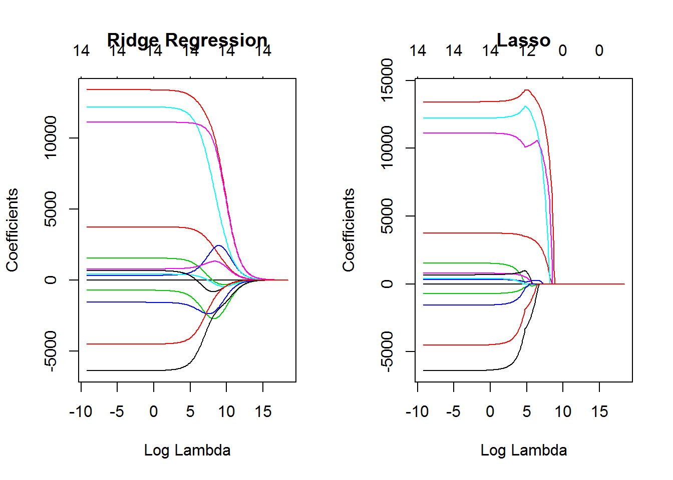

Here is a calculation to determine the best lambda for the two methods:

ridge.cv <- cv.glmnet(cars_train_mat, cars_train$Price, alpha = 0)
lambda_ridge <- ridge.cv$lambda.min
lambda_ridge

## [1] 736.0895

lasso.cv <- cv.glmnet(cars_train_mat, cars_train$Price, alpha = 1)
lambda_lasso <- lasso.cv$lambda.min
lambda_lasso

## [1] 10.93069

Again we’ll compare the new MSE:

cars_test_mat <- model.matrix(Price ~ . -Saturn, cars_test)[,-1]
cars_ridge_predictions <- predict(cars_models_ridge, s = lambda_ridge, newx = cars_test_mat)
compute_mse(cars_ridge_predictions, cars_test$Price)

## [1] 6576660

cars_lasso_predictions <- predict(cars_models_lasso, s = lambda_lasso, newx = cars_test_mat)
compute_mse(cars_lasso_predictions, cars_test$Price)

## [1] 6615395

11 Conclusion

We have seen how to significantly improve the performance of linear models.

Source

Miller, J. D., & Forte, R. M. (2017). Mastering Predictive Analytics with R. Packt Publishing Ltd.