Table of Content

• 1 Introduction
• 2 Preparation
• 3 k-Means
• 3.1 Choosing k
• 4 Hierachical clustering
• 5 Model based clustering
• 6 Density based clustering
• 7 Conclusion

1 Introduction

The cluster analysis groups examination objects into natural groups (so-called “clusters”). The objects to be examined may be individuals, objects as well as countries or organizations. By applying cluster analytic methods, these objects can be clustered by their properties. Each cluster should be as homogeneous as possible while the clusters should be as different as possible.

Cluster analytical methods have an exploratory character, since one does not make any inferential statistical conclusions about the population, but rather tries to discover a structure in a data-driven manner. The researchers play an important role in this, since the result is influenced, among other things, by the choice of the clustering algorithm.

The question of cluster analysis is often shortened as follows: “Can the objects being examined be combined into natural clusters?”

For this post the dataset Iris_Data from the statistic platform “Kaggle” was used. A copy of the record is available at https://drive.google.com/open?id=12zICkGCSYfsptsgpdSJeWRvRwULq6ftc.

2 Preparation

To perform a cluster analysis in R, generally, the data should be prepared as follows:

• Rows are observations (individuals) and columns are variables
• Any missing value in the data must be removed or estimated.
• The data must be standardized (i.e., scaled) to make variables comparable.

iris$species <- as.factor(iris$species)
irisScaled <- scale(iris[, -5])
sum(is.na(irisScaled))

## [1] 0

In the following, several cluster methods will be presented.

3 k-Means

fitK <- kmeans(irisScaled, centers = 3, nstart = 25)
fitK

## K-means clustering with 3 clusters of sizes 53, 47, 50
## 
## Cluster means:
##   sepal_length sepal_width petal_length petal_width
## 1  -0.05005221  -0.8773526    0.3463713   0.2811215
## 2   1.13217737   0.0962759    0.9929445   1.0137756
## 3  -1.01119138   0.8394944   -1.3005215  -1.2509379
## 
## Clustering vector:
##   [1] 3 3 3 3 3 3 3 3 3 3 3 3 3 3 3 3 3 3 3 3 3 3 3 3 3 3 3 3 3 3 3 3 3 3 3
##  [36] 3 3 3 3 3 3 3 3 3 3 3 3 3 3 3 2 2 2 1 1 1 2 1 1 1 1 1 1 1 1 2 1 1 1 1
##  [71] 2 1 1 1 1 2 2 2 1 1 1 1 1 1 1 2 2 1 1 1 1 1 1 1 1 1 1 1 1 1 2 1 2 2 2
## [106] 2 1 2 2 2 2 2 2 1 1 2 2 2 2 1 2 1 2 1 2 2 1 2 2 2 2 2 2 1 1 2 2 2 1 2
## [141] 2 2 1 2 2 2 1 2 2 1
## 
## Within cluster sum of squares by cluster:
## [1] 44.25778 47.60995 48.15831
##  (between_SS / total_SS =  76.5 %)
## 
## Available components:
## 
## [1] "cluster"      "centers"      "totss"        "withinss"    
## [5] "tot.withinss" "betweenss"    "size"         "iter"        
## [9] "ifault"

plot(iris, col = fitK$cluster)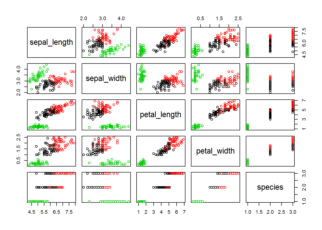

3.1 Choosing k

There are several ways to determine the number of k. One option is to do this via visualization.

fitK3 <- kmeans(irisScaled, centers = 4, nstart = 25)
fitK4 <- kmeans(irisScaled, centers = 5, nstart = 25)
fitK5 <- kmeans(irisScaled, centers = 6, nstart = 25)

# plots to compare
p1 <- fviz_cluster(fitK, geom = "point", data = irisScaled) + ggtitle("k = 3")
p2 <- fviz_cluster(fitK3, geom = "point",  data = irisScaled) + ggtitle("k = 4")
p3 <- fviz_cluster(fitK4, geom = "point",  data = irisScaled) + ggtitle("k = 5")
p4 <- fviz_cluster(fitK5, geom = "point",  data = irisScaled) + ggtitle("k = 6")


grid.arrange(p1, p2, p3, p4, nrow = 2)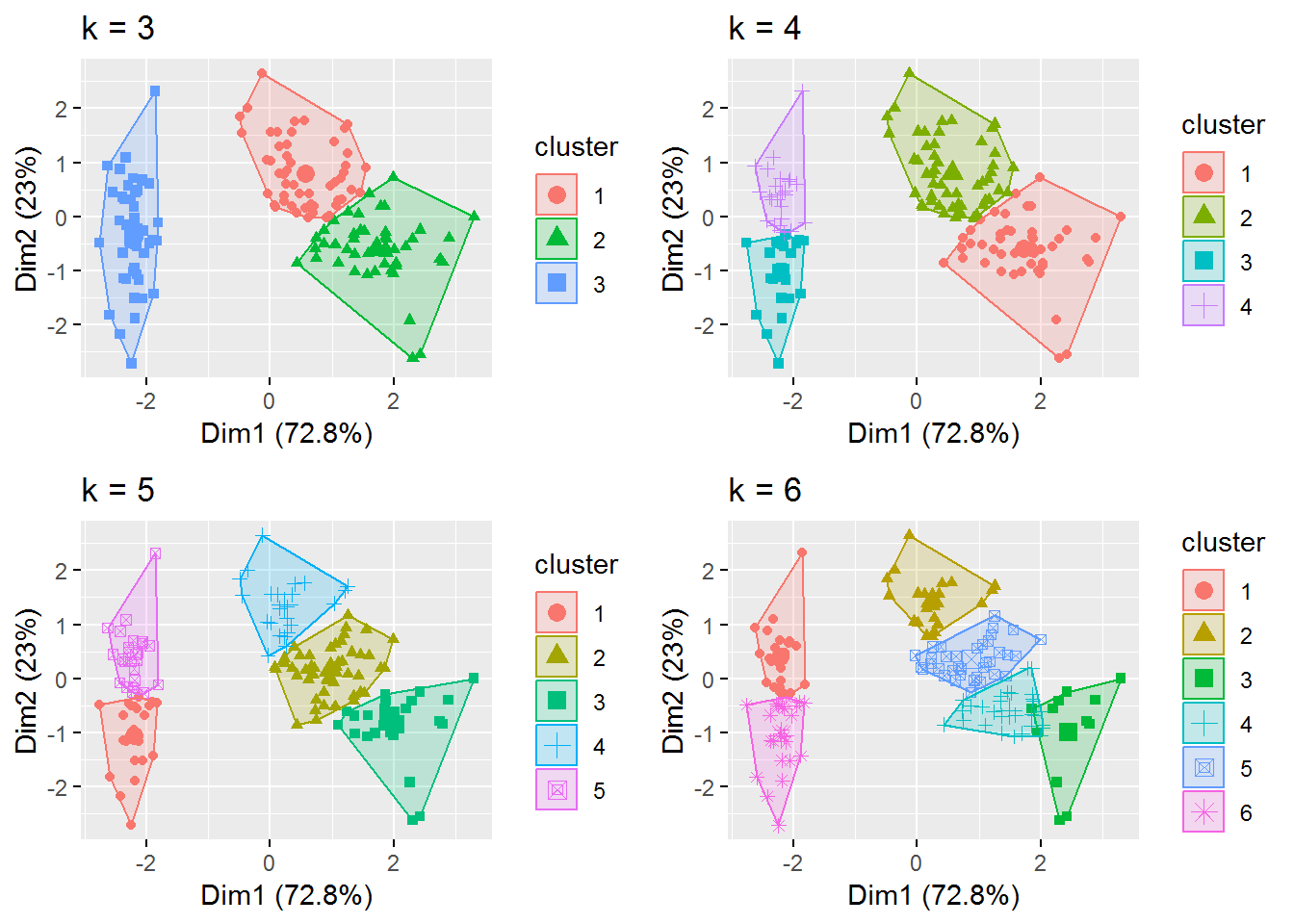

Another possibility would be to look at the outputs of different variants for k. The following example calculates k Means for k: 1 to 5.

k <- list()
for(i in 1:5){
  k[[i]] <- kmeans(irisScaled, i)
}

k

## [[1]]
## K-means clustering with 1 clusters of sizes 150
## 
## Cluster means:
##    sepal_length  sepal_width  petal_length  petal_width
## 1 -9.793092e-16 4.455695e-16 -4.988602e-16 1.206442e-16
## 
## Clustering vector:
##   [1] 1 1 1 1 1 1 1 1 1 1 1 1 1 1 1 1 1 1 1 1 1 1 1 1 1 1 1 1 1 1 1 1 1 1 1
##  [36] 1 1 1 1 1 1 1 1 1 1 1 1 1 1 1 1 1 1 1 1 1 1 1 1 1 1 1 1 1 1 1 1 1 1 1
##  [71] 1 1 1 1 1 1 1 1 1 1 1 1 1 1 1 1 1 1 1 1 1 1 1 1 1 1 1 1 1 1 1 1 1 1 1
## [106] 1 1 1 1 1 1 1 1 1 1 1 1 1 1 1 1 1 1 1 1 1 1 1 1 1 1 1 1 1 1 1 1 1 1 1
## [141] 1 1 1 1 1 1 1 1 1 1
## 
## Within cluster sum of squares by cluster:
## [1] 596
##  (between_SS / total_SS =   0.0 %)
## 
## Available components:
## 
## [1] "cluster"      "centers"      "totss"        "withinss"    
## [5] "tot.withinss" "betweenss"    "size"         "iter"        
## [9] "ifault"      
## 
## [[2]]
## K-means clustering with 2 clusters of sizes 50, 100
## 
## Cluster means:
##   sepal_length sepal_width petal_length petal_width
## 1   -1.0111914   0.8394944   -1.3005215  -1.2509379
## 2    0.5055957  -0.4197472    0.6502607   0.6254689
## 
## Clustering vector:
##   [1] 1 1 1 1 1 1 1 1 1 1 1 1 1 1 1 1 1 1 1 1 1 1 1 1 1 1 1 1 1 1 1 1 1 1 1
##  [36] 1 1 1 1 1 1 1 1 1 1 1 1 1 1 1 2 2 2 2 2 2 2 2 2 2 2 2 2 2 2 2 2 2 2 2
##  [71] 2 2 2 2 2 2 2 2 2 2 2 2 2 2 2 2 2 2 2 2 2 2 2 2 2 2 2 2 2 2 2 2 2 2 2
## [106] 2 2 2 2 2 2 2 2 2 2 2 2 2 2 2 2 2 2 2 2 2 2 2 2 2 2 2 2 2 2 2 2 2 2 2
## [141] 2 2 2 2 2 2 2 2 2 2
## 
## Within cluster sum of squares by cluster:
## [1]  48.15831 174.08215
##  (between_SS / total_SS =  62.7 %)
## 
## Available components:
## 
## [1] "cluster"      "centers"      "totss"        "withinss"    
## [5] "tot.withinss" "betweenss"    "size"         "iter"        
## [9] "ifault"      
## 
## [[3]]
## K-means clustering with 3 clusters of sizes 50, 47, 53
## 
## Cluster means:
##   sepal_length sepal_width petal_length petal_width
## 1  -1.01119138   0.8394944   -1.3005215  -1.2509379
## 2   1.13217737   0.0962759    0.9929445   1.0137756
## 3  -0.05005221  -0.8773526    0.3463713   0.2811215
## 
## Clustering vector:
##   [1] 1 1 1 1 1 1 1 1 1 1 1 1 1 1 1 1 1 1 1 1 1 1 1 1 1 1 1 1 1 1 1 1 1 1 1
##  [36] 1 1 1 1 1 1 1 1 1 1 1 1 1 1 1 2 2 2 3 3 3 2 3 3 3 3 3 3 3 3 2 3 3 3 3
##  [71] 2 3 3 3 3 2 2 2 3 3 3 3 3 3 3 2 2 3 3 3 3 3 3 3 3 3 3 3 3 3 2 3 2 2 2
## [106] 2 3 2 2 2 2 2 2 3 3 2 2 2 2 3 2 3 2 3 2 2 3 2 2 2 2 2 2 3 3 2 2 2 3 2
## [141] 2 2 3 2 2 2 3 2 2 3
## 
## Within cluster sum of squares by cluster:
## [1] 48.15831 47.60995 44.25778
##  (between_SS / total_SS =  76.5 %)
## 
## Available components:
## 
## [1] "cluster"      "centers"      "totss"        "withinss"    
## [5] "tot.withinss" "betweenss"    "size"         "iter"        
## [9] "ifault"      
## 
## [[4]]
## K-means clustering with 4 clusters of sizes 22, 29, 49, 50
## 
## Cluster means:
##   sepal_length sepal_width petal_length petal_width
## 1   -0.4201099  -1.4244568   0.03888306  -0.0518577
## 2    1.3926646   0.2412870   1.15694270   1.2126820
## 3   -0.9987207   0.8921158  -1.29862458  -1.2524354
## 4    0.3558492  -0.3874590   0.58451677   0.5468485
## 
## Clustering vector:
##   [1] 3 3 3 3 3 3 3 3 3 3 3 3 3 3 3 3 3 3 3 3 3 3 3 3 3 3 3 3 3 3 3 3 3 3 3
##  [36] 3 3 3 3 3 3 1 3 3 3 3 3 3 3 3 2 4 2 1 4 4 4 1 4 1 1 4 1 4 4 4 4 1 1 1
##  [71] 4 4 4 4 4 4 4 4 4 1 1 1 1 4 4 4 4 1 4 1 1 4 1 1 1 4 4 4 1 4 2 4 2 4 2
## [106] 2 1 2 4 2 2 4 2 4 4 2 4 2 2 1 2 4 2 4 2 2 4 4 4 2 2 2 4 4 4 2 2 4 4 2
## [141] 2 2 4 2 2 2 4 4 2 4
## 
## Within cluster sum of squares by cluster:
## [1] 17.08819 26.99662 40.97891 29.68156
##  (between_SS / total_SS =  80.7 %)
## 
## Available components:
## 
## [1] "cluster"      "centers"      "totss"        "withinss"    
## [5] "tot.withinss" "betweenss"    "size"         "iter"        
## [9] "ifault"      
## 
## [[5]]
## K-means clustering with 5 clusters of sizes 26, 24, 29, 23, 48
## 
## Cluster means:
##   sepal_length sepal_width petal_length petal_width
## 1   -1.2971217   0.2036643   -1.3040964 -1.29347351
## 2   -0.7014335   1.5283103   -1.2966486 -1.20485757
## 3    1.3926646   0.2412870    1.1569427  1.21268196
## 4   -0.3516137  -1.3278291    0.1022793  0.01314138
## 5    0.3804044  -0.3839995    0.6067148  0.56410134
## 
## Clustering vector:
##   [1] 2 1 1 1 2 2 1 1 1 1 2 1 1 1 2 2 2 2 2 2 2 2 2 1 1 1 1 2 2 1 1 2 2 2 1
##  [36] 1 2 1 1 1 2 1 1 2 2 1 2 1 2 1 3 5 3 4 5 5 5 4 5 4 4 5 4 5 4 5 5 4 4 4
##  [71] 5 5 5 5 5 5 5 5 5 4 4 4 4 5 5 5 5 4 5 4 4 5 4 4 4 5 5 5 4 4 3 5 3 5 3
## [106] 3 4 3 5 3 3 5 3 5 5 3 5 3 3 4 3 5 3 5 3 3 5 5 5 3 3 3 5 5 5 3 3 5 5 3
## [141] 3 3 5 3 3 3 5 5 3 5
## 
## Within cluster sum of squares by cluster:
## [1]  9.803125 11.929538 26.996617 13.745359 27.921119
##  (between_SS / total_SS =  84.8 %)
## 
## Available components:
## 
## [1] "cluster"      "centers"      "totss"        "withinss"    
## [5] "tot.withinss" "betweenss"    "size"         "iter"        
## [9] "ifault"

Another option is the “elbow” method.

betweenss_totss <- list()
for(i in 1:5){
  betweenss_totss[[i]] <- k[[i]]$betweenss/k[[i]]$totss
}

plot(1:5, betweenss_totss, type = "b", ylab = "Between SS / Total SS", xlab = "Cluster (k)")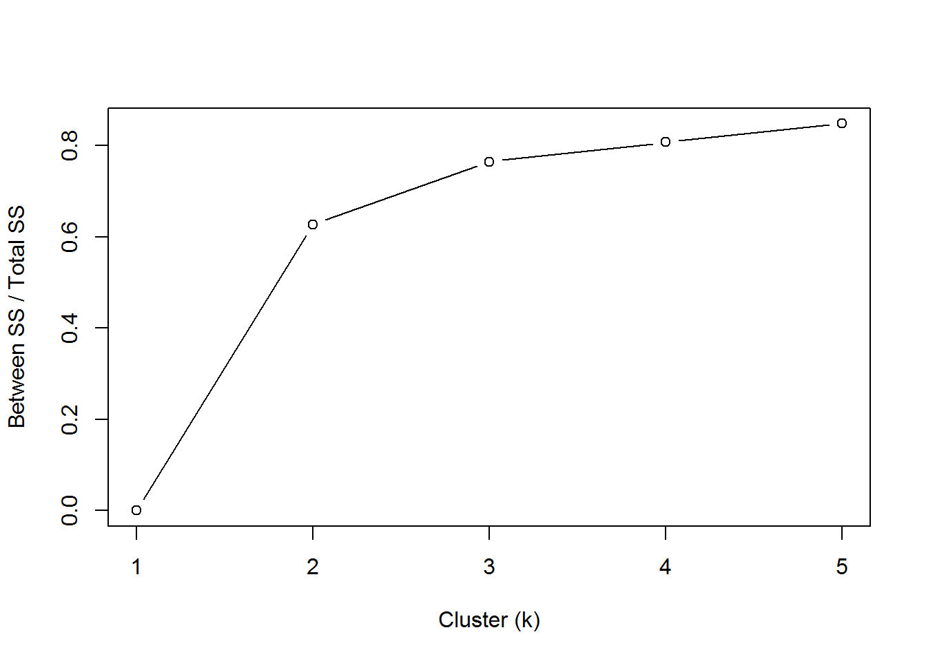

Average Silhouette Method

fviz_nbclust(irisScaled, kmeans, method = "silhouette")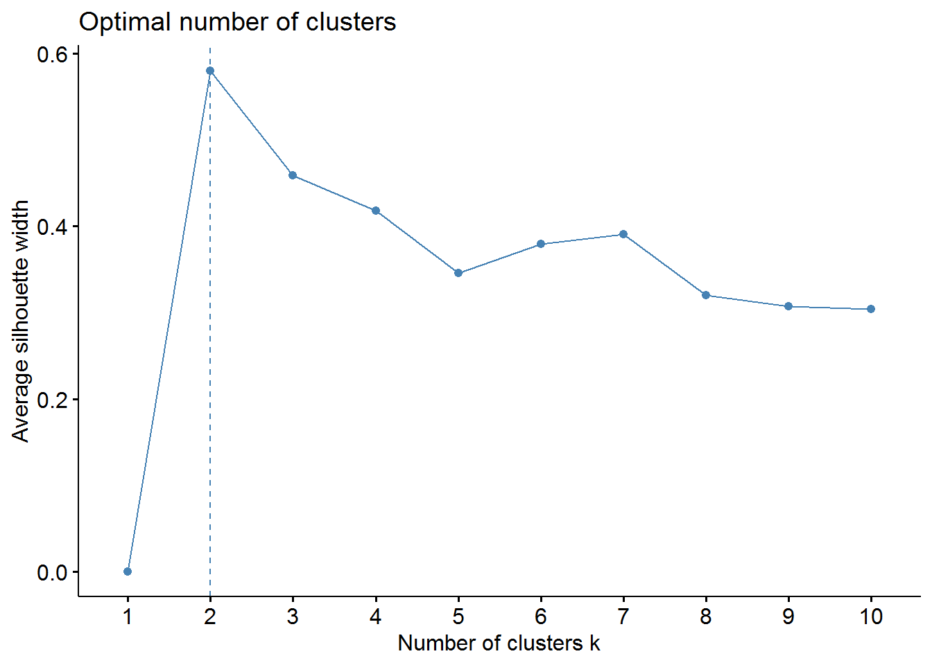

Gap Statistic Method

set.seed(123)
gap_stat <- clusGap(irisScaled, FUN = kmeans, nstart = 25,
                    K.max = 10, B = 50)

fviz_gap_stat(gap_stat)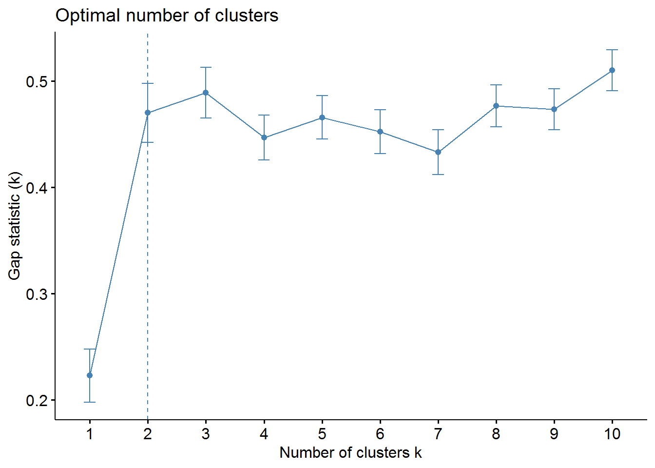

It can be seen that the results for k fall differently. From that I advise always different methods to test.

Here we can see the final result with k=3.

fviz_cluster(fitK, data = irisScaled)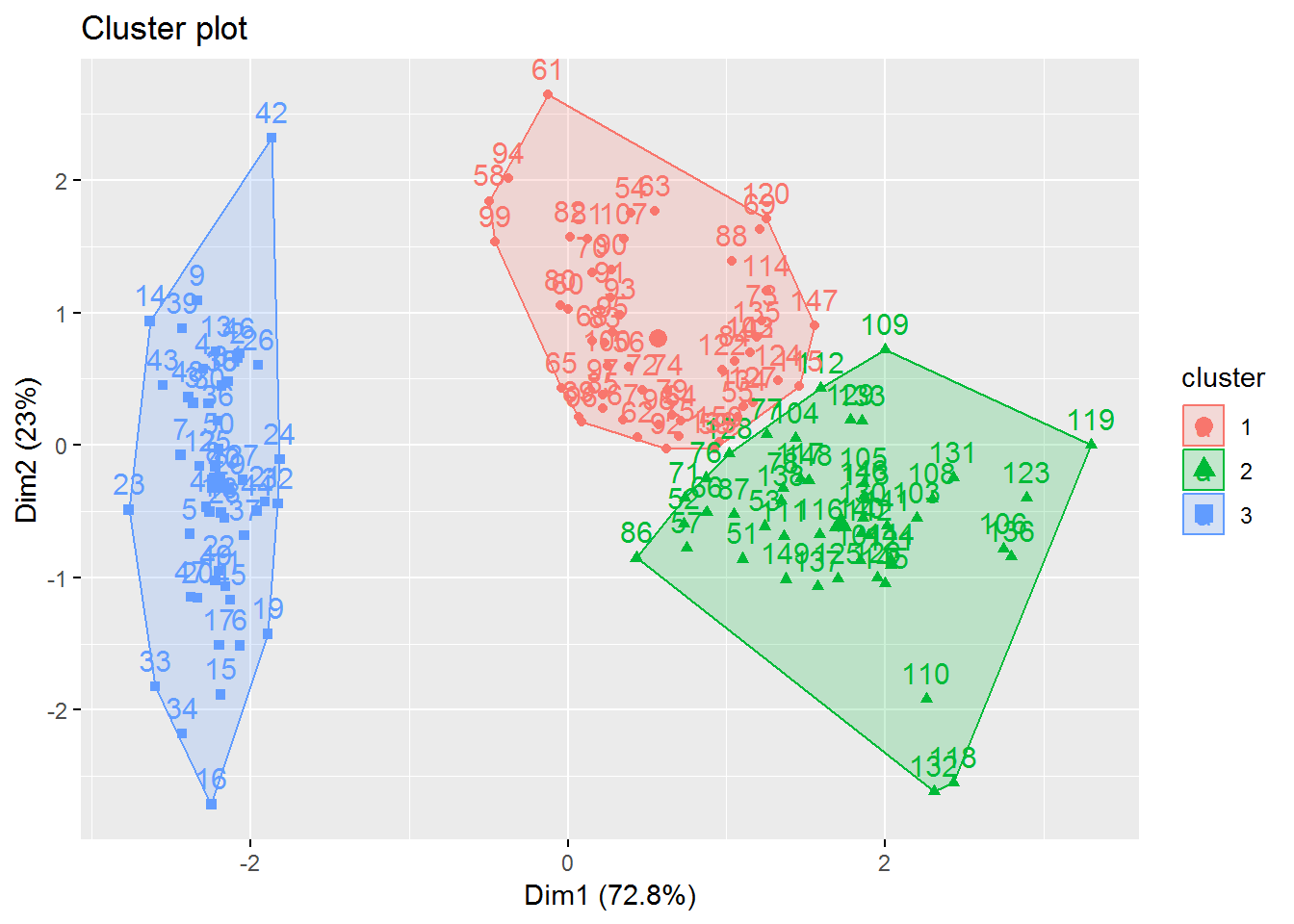

3.2 Transfer the found clusters

The corresponding assignment of the found clusters should now be transferred to the original data record.

out <- cbind(iris, clusterNum = fitK$cluster)
head(out)

##   sepal_length sepal_width petal_length petal_width     species clusterNum
## 1          5.1         3.5          1.4         0.2 Iris-setosa          3
## 2          4.9         3.0          1.4         0.2 Iris-setosa          3
## 3          4.7         3.2          1.3         0.2 Iris-setosa          3
## 4          4.6         3.1          1.5         0.2 Iris-setosa          3
## 5          5.0         3.6          1.4         0.2 Iris-setosa          3
## 6          5.4         3.9          1.7         0.4 Iris-setosa          3

4 Hierachical clustering

Hierarchical clustering involves creating clusters that have a predetermined ordering from top to bottom.

d <- dist(irisScaled)

fitH <- hclust(d, "ward.D")
plot(fitH)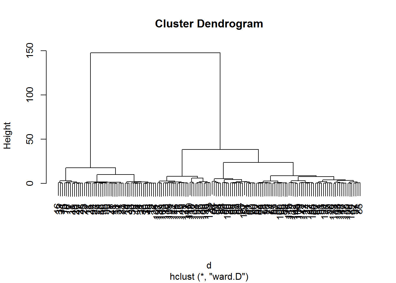

clusters <- cutree(fitH, 3)
plot(iris, col = clusters)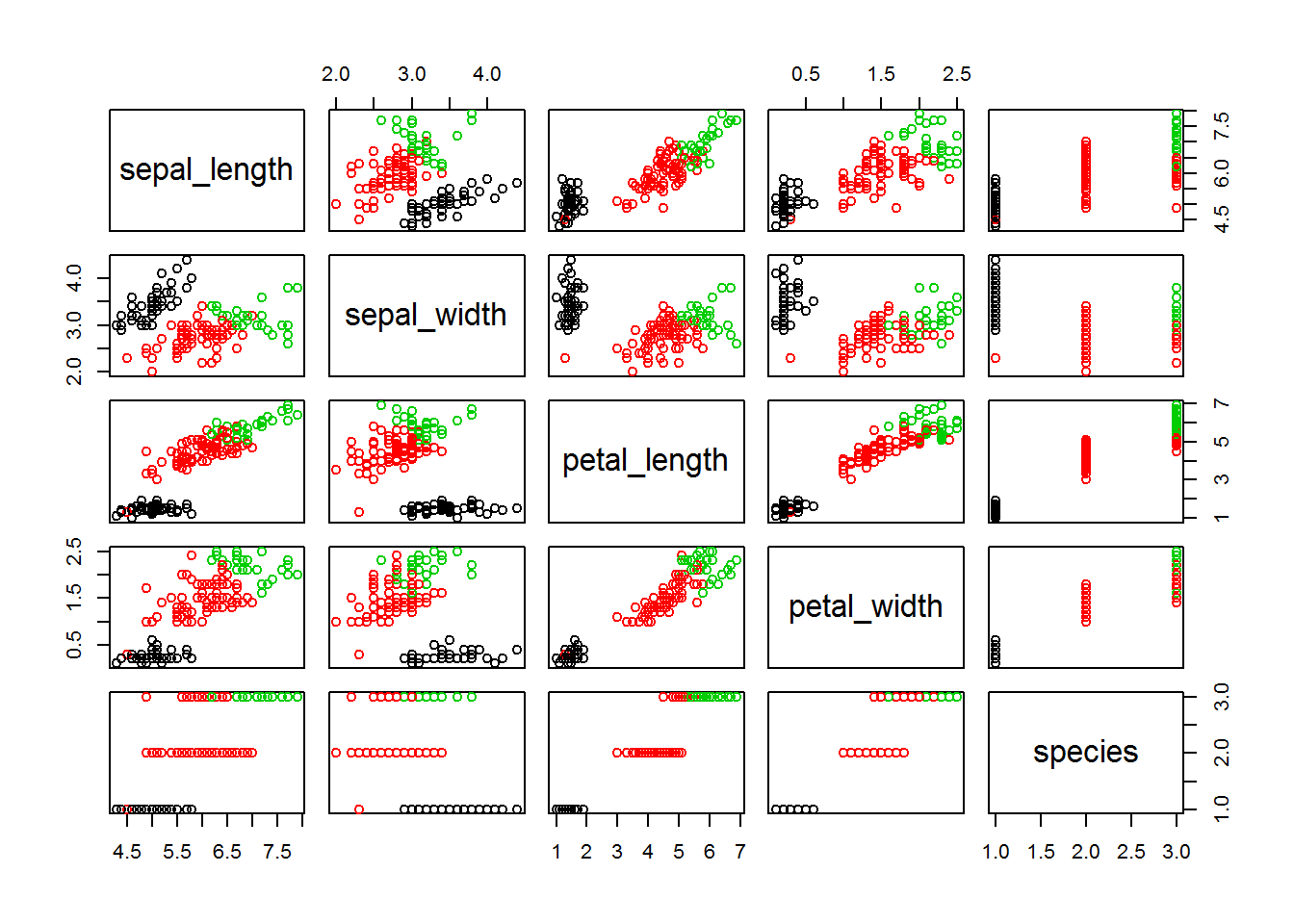

5 Model based clustering

The traditional clustering methods, such as hierarchical clustering and k-means clustering, are heuristic and are not based on formal models. Furthermore, k-means algorithm is commonly randomnly initialized, so different runs of k-means will often yield different results. Additionally, k-means requires the user to specify the the optimal number of clusters.

An alternative is model-based clustering, which consider the data as coming from a distribution that is mixture of two or more clusters. Unlike k-means, the model-based clustering uses a soft assignment, where each data point has a probability of belonging to each cluster.

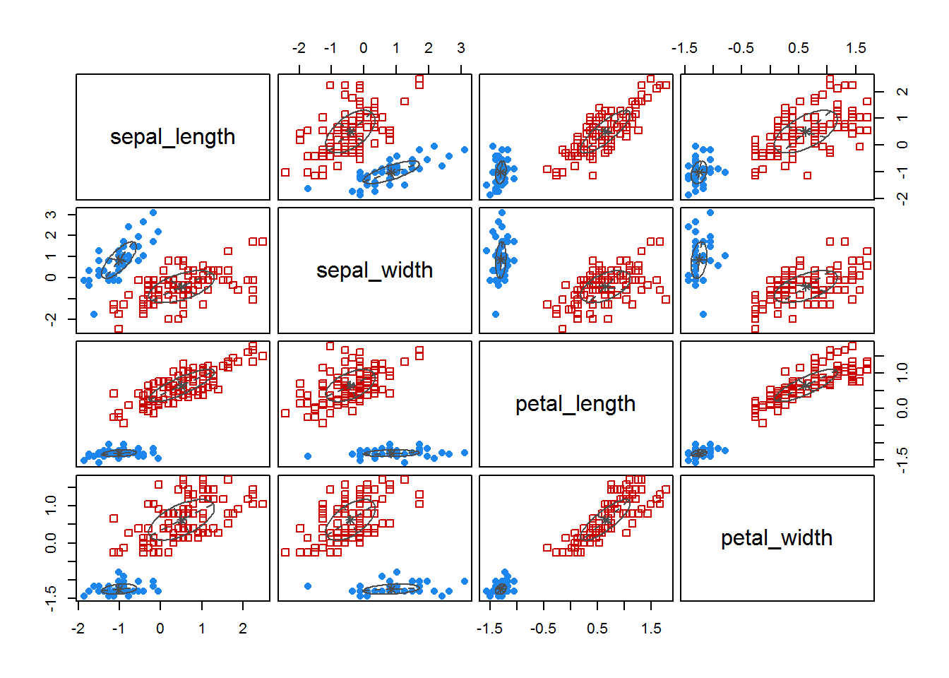
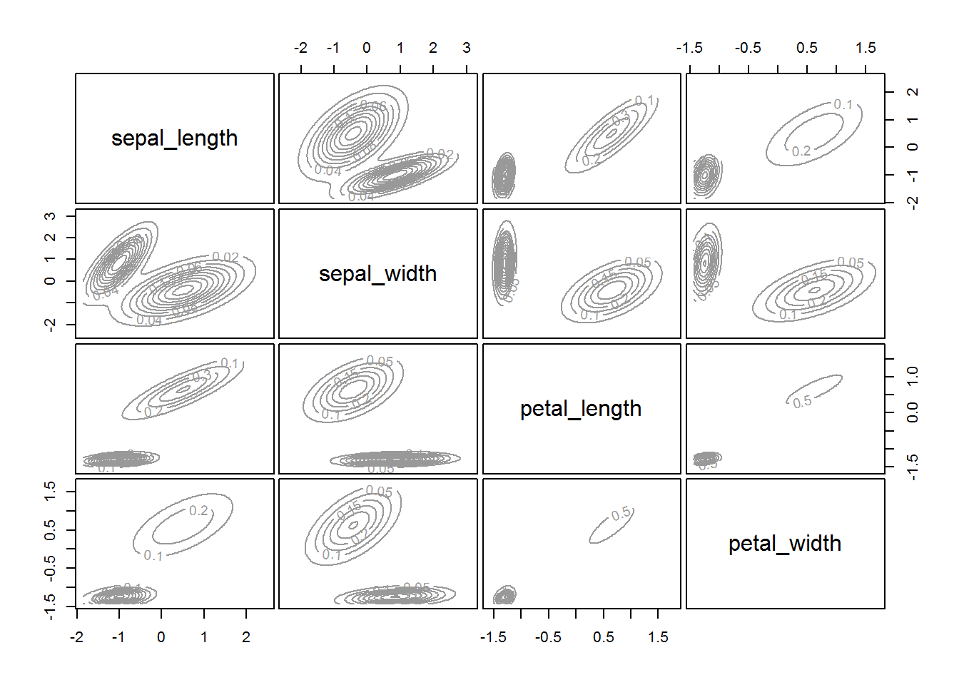
fitM <- Mclust(irisScaled)
fitM

plot(fitM)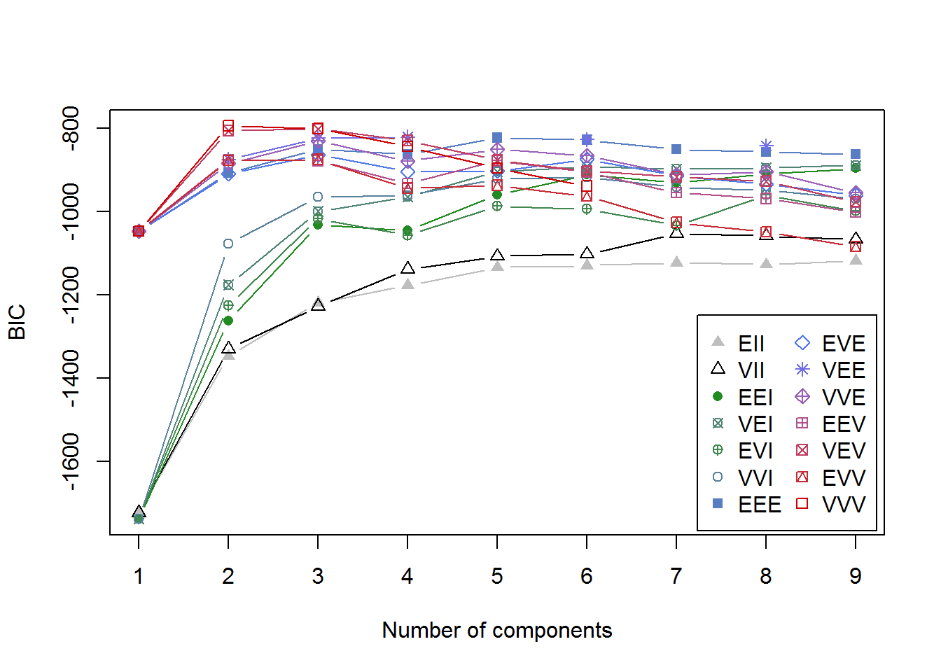

6 Density based clustering

The Density-Based Clustering tool works by detecting areas where points are concentrated and separated by empty and low-density areas. Points that are not part of a cluster are marked as noise. This tool uses unsupervised machine learning clustering algorithms that automatically detect patterns based on purely spatial locations and the distance to a specified number of neighbors.

kNNdistplot(irisScaled, k = 3)
abline(h = 0.7, col = "red", lty = 2)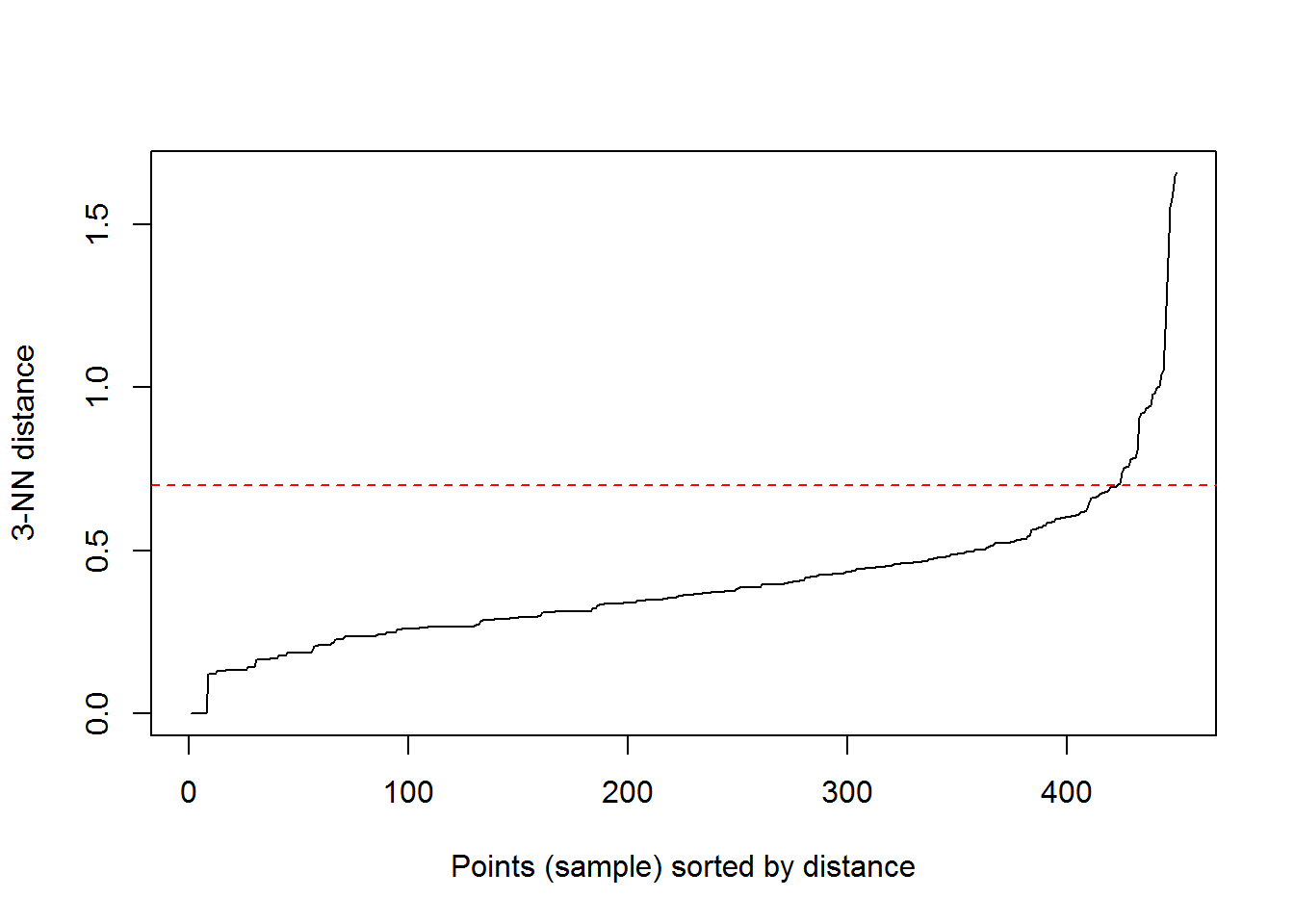

fitD <- dbscan(irisScaled, eps = 0.7, minPts = 5)
fitD

## DBSCAN clustering for 150 objects.
## Parameters: eps = 0.7, minPts = 5
## The clustering contains 2 cluster(s) and 8 noise points.
## 
##  0  1  2 
##  8 48 94 
## 
## Available fields: cluster, eps, minPts

plot(iris, col = fitD$cluster)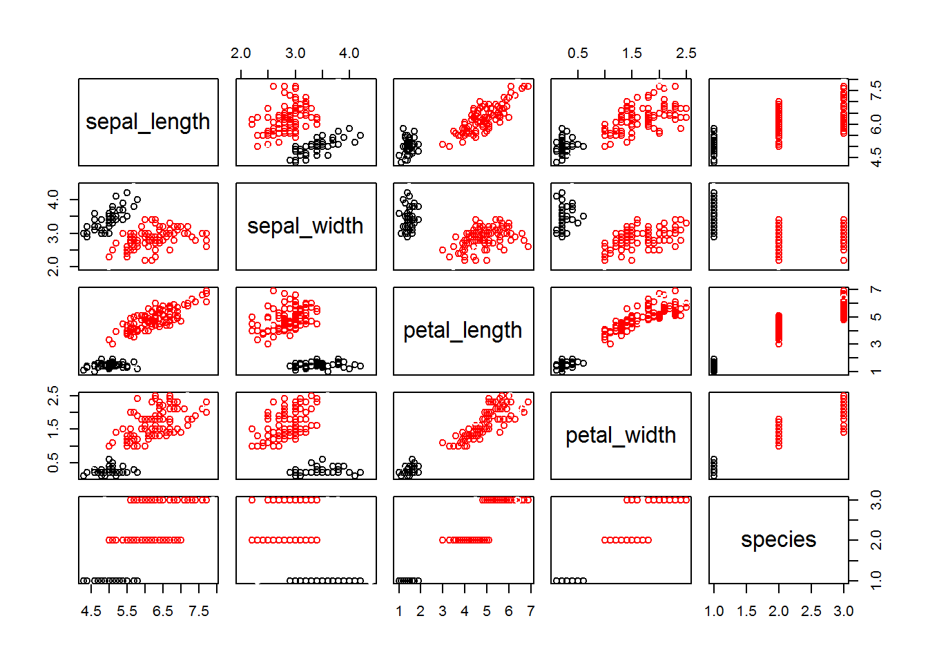

7 Conclusion

In this post several types of clustering methods were shown. As the last example shows, not every algorithm is suitable for every record. From this point of view, you should always try several options in order to finally choose the best algorithm for your data.