Table of Content

• 1 Introduction
• 2 The way LDA works
• 3 PCA vs. LDA
• 4 Closing word

1 Introduction

Linear discriminant analysis (LDA) is a type of linear combination, a mathematical process using various data items and applying functions to that set to separately analyze multiple classes of objects or items. LDA is most commonly used as dimensionality reduction technique in the pre-processing step for pattern-classification and machine learning applications. The main target is to project a dataset onto a lower-dimensional space with good class-separability in order avoid overfitting and also reduce computational costs.

For this post the dataset Iris_Data from the statistic platform “Kaggle” was used. A copy of the record is available at https://drive.google.com/open?id=12zICkGCSYfsptsgpdSJeWRvRwULq6ftc.

2 The way LDA works

The general LDA approach is very similar to a Principal Component Analysis, but in addition to finding the component axes that maximize the variance of our data (PCA), we are additionally interested in the axes that maximize the separation between multiple classes (LDA).

As a first step we need to establish what the prior distribution of data is.

table(iris$species)

## 
##     Iris-setosa Iris-versicolor  Iris-virginica 
##              50              50              50

Here there are three classes, all equally distributed. The prior distirbution in this case would be 1/3 for each class.

iris.LDA <- lda(species ~ ., data = iris, prior = c(1/3, 1/3, 1/3))
iris.LDA

## Call:
## lda(species ~ ., data = iris, prior = c(1/3, 1/3, 1/3))
## 
## Prior probabilities of groups:
##     Iris-setosa Iris-versicolor  Iris-virginica 
##       0.3333333       0.3333333       0.3333333 
## 
## Group means:
##                 sepal_length sepal_width petal_length petal_width
## Iris-setosa            5.006       3.418        1.464       0.244
## Iris-versicolor        5.936       2.770        4.260       1.326
## Iris-virginica         6.588       2.974        5.552       2.026
## 
## Coefficients of linear discriminants:
##                     LD1         LD2
## sepal_length  0.8192685  0.03285975
## sepal_width   1.5478732  2.15471106
## petal_length -2.1849406 -0.93024679
## petal_width  -2.8538500  2.80600460
## 
## Proportion of trace:
##    LD1    LD2 
## 0.9915 0.0085

The output here shows that the first value (LD1) describes 99% of the variance in the data and the other one (LD2) 0.8%.Another way to calculate this would be:

iris.LDA$svd^2/sum(iris.LDA$svd^2)

## [1] 0.991472476 0.008527524

Here you can see how the two linear discriminants are related to each of the features in the data:

iris.LDA$scaling

##                     LD1         LD2
## sepal_length  0.8192685  0.03285975
## sepal_width   1.5478732  2.15471106
## petal_length -2.1849406 -0.93024679
## petal_width  -2.8538500  2.80600460

Now we’ll have a look how well the LDA model compares with the actual answers for the iris species data:

iris.LDA.prediction <- predict(iris.LDA, newdata = iris)
table(iris.LDA.prediction$class, iris$species)

##                  
##                   Iris-setosa Iris-versicolor Iris-virginica
##   Iris-setosa              50               0              0
##   Iris-versicolor           0              48              1
##   Iris-virginica            0               2             49

3 PCA vs. LDA

The last step is to compare the two models (PCA and LDA). As a note: PCA is an unsupervised learner and LDA a supervised one. Supervised models will tend to be better at separating data than unsupervised ones. Let’s see which model has better geared.

iris.PCA <- prcomp(iris[, -5], center = T, scale. = T)

combined.methods <- data.frame(species = iris[, "species"], pca = iris.PCA$x, lda = iris.LDA.prediction$x)

LDA.plot <- ggplot(combined.methods) + 
  geom_point(aes(lda.LD1, lda.LD2, shape = species, color = species)) + 
  scale_shape_manual(values = c(0, 1, 2)) +
  ggtitle("Classification with LDA")


PCA.plot <- ggplot(combined.methods) + 
  geom_point(aes(pca.PC1, pca.PC2, shape = species, color = species)) + 
  scale_shape_manual(values = c(0, 1, 2)) +
  ggtitle("Classification with PCA")

grid.arrange(PCA.plot, LDA.plot)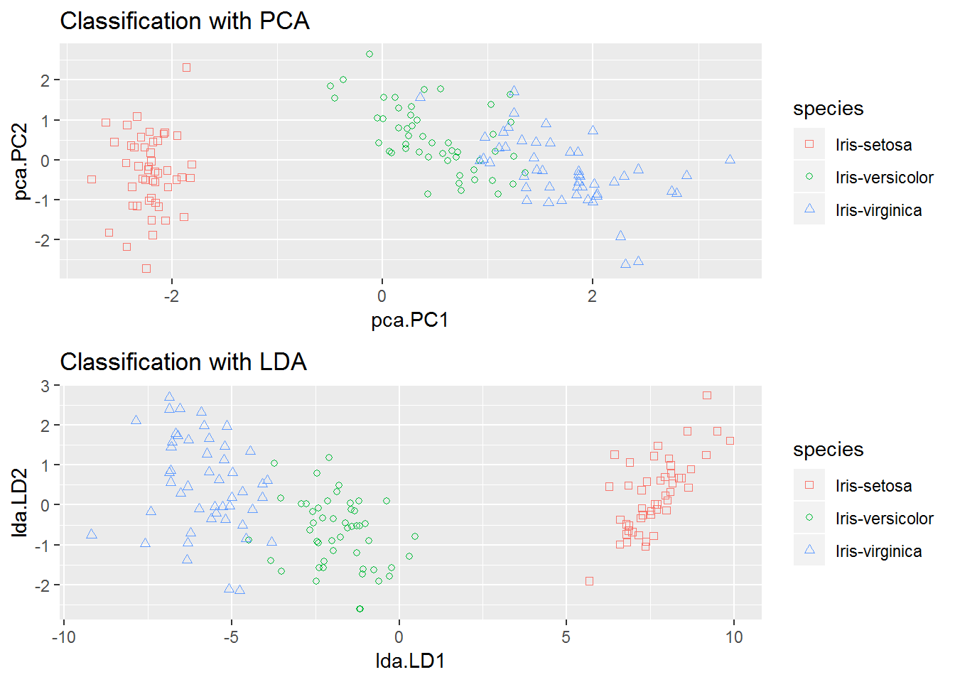

In both models the setosa data is well separated from the rest, but it looks like LDA performs better at keeping the overlap between versicolor and virginica to a minimum.

4 Closing word

Principal Component Analysis vs. Linear Discriminant Analysis:

Both Linear Discriminant Analysis and Principal Component Analysis are linear transformation techniques that are commonly used for dimensionality reduction. PCA can be described as an unsupervised algorithm, since it ignores class labels and its goal is to find the directions that maximize the variance in a dataset. In contrast to PCA, LDA is supervised and computes the directions that will represent the axes that that maximize the separation between multiple classes. Although it might sound intuitive that LDA is superior to PCA for a multi-class classification task where the class labels are known, this might not always the case. In practice, it is also not uncommon to use both LDA and PCA in combination: E.g., PCA for dimensionality reduction followed by an LDA.

Source

Burger, S. V. (2018). Introduction to Machine Learning with R: Rigorous Mathematical Analysis. " O’Reilly Media, Inc.“.