library(tidyverse)mtcars <- read_csv("mtcars.csv")Table of Content
- 1 Introduction
- 2 The way PCA works
- 3 Closing word
1 Introduction
Principal Component Analysis (PCA) is used when you want to structure or simplify a large data set. An attempt is made to reduce the total number of measured variables while still accounting for the largest possible portion of the variance of all variables. The PCA works purely exploratory and searches in the data for a linear pattern that best describes the data set.
One of the biggest problems with multivariate data is that they can not be displayed two-dimensionally, so they can not be displayed on the computer screen. The more variables a record has, the more complicated the situation becomes. This leads to the fact that one no longer recognizes existing relationships. The central idea of the principal component analysis is now to project the data onto a two-dimensional plane in such a way that the required relationships become visible. The visible structure of the projected data depends on the direction of the projection.
For this post the dataset mtcars from the statistic platform “Kaggle” was used. A copy of the record is available at https://drive.google.com/open?id=1u7cDZoOUg9ah8ZG3aiUWmUgts8RTL4iR.
2 The way PCA works
PCA’s usefulness for dimensionality reduction of data can be helpful for visualizing complex data patterns. The example below is intended to illustrate this.
head(mtcars)## # A tibble: 6 x 12
## X1 mpg cyl disp hp drat wt qsec vs am gear carb
## <chr> <dbl> <int> <dbl> <int> <dbl> <dbl> <dbl> <int> <int> <int> <int>
## 1 Mazda~ 21 6 160 110 3.9 2.62 16.5 0 1 4 4
## 2 Mazda~ 21 6 160 110 3.9 2.88 17.0 0 1 4 4
## 3 Datsu~ 22.8 4 108 93 3.85 2.32 18.6 1 1 4 1
## 4 Horne~ 21.4 6 258 110 3.08 3.22 19.4 1 0 3 1
## 5 Horne~ 18.7 8 360 175 3.15 3.44 17.0 0 0 3 2
## 6 Valia~ 18.1 6 225 105 2.76 3.46 20.2 1 0 3 1Let’s have a look which features of the mtcars dataset might be correlated with one another.
pairs(mtcars[, 2:8], lower.panel = NULL)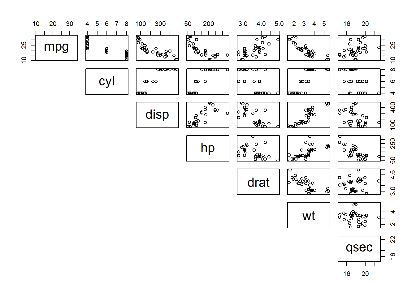
At first glance of the data, it looks like there are some well-correlated values, with many of them corresponding to the vehicle’s weight variable (wt).
Now we are trying to reduce some of these variables’dependencies and generate a more simplified picture of the data.
PCA <- princomp(mtcars[, 2:8], scores = TRUE, cor = TRUE)
summary(PCA)
## Importance of components:
## Comp.1 Comp.2 Comp.3 Comp.4 Comp.5
## Standard deviation 2.2552383 1.0754374 0.5872406 0.39740859 0.35985282
## Proportion of Variance 0.7265857 0.1652236 0.0492645 0.02256194 0.01849915
## Cumulative Proportion 0.7265857 0.8918093 0.9410738 0.96363579 0.98213494
## Comp.6 Comp.7
## Standard deviation 0.27542160 0.22180708
## Proportion of Variance 0.01083672 0.00702834
## Cumulative Proportion 0.99297166 1.00000000This table shows how important each of these principal components are to the overall dataset. We can also plot this.
plot(PCA)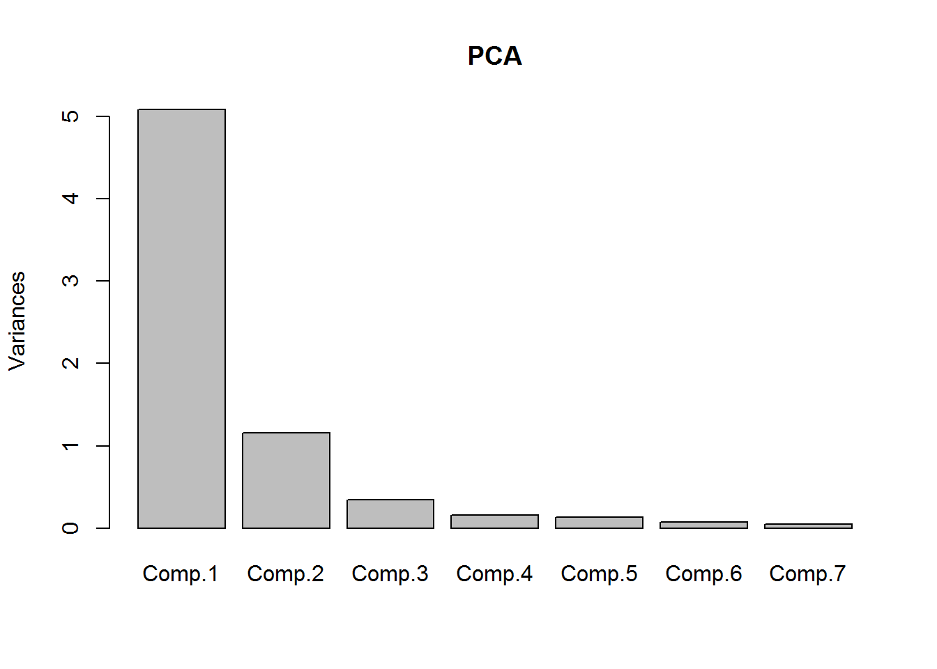
We can see Comp.1 + Comp.2 explains upward of 89% of the dataset with just two features instead of 7 that we started with. But what does Comp.1 and so on mean to us?
PCA$loadings[, 1:5]## Comp.1 Comp.2 Comp.3 Comp.4 Comp.5
## mpg 0.4127573 0.08296098 0.2416477 0.766798834 0.2127946
## cyl -0.4247315 0.07844163 0.1880252 0.193926827 -0.2383825
## disp -0.4225036 -0.08239922 -0.1180359 0.587679498 -0.1488730
## hp -0.3877611 0.33696384 -0.2027400 -0.006884691 0.8314576
## drat 0.3311703 0.44858845 -0.7552915 0.117073263 -0.2217502
## wt -0.3913153 -0.32236122 -0.4405532 0.107346915 -0.1666473
## qsec 0.2399275 -0.74932087 -0.2943885 0.061382684 0.3278152Since only Comp.1 and 2 are relevant for the further analysis, the following step focuses only on these two components.
Now we are looking for the dominant positive or negative value within these components:
- Comp.1 is correlated to mpg and cyl
- Comp.2 is correlated to qsec, gear and am
If you wanted to see this kind of information in a more graphical sence, you can plot the scores of the principal components as shown in the following graphic.
scores.df <- data.frame(PCA$scores)
scores.df$No <- row.names(scores.df)
mtcars$No <- row.names(mtcars)
scores.df.new <- merge(scores.df, mtcars, by = "No")
plot(x = scores.df.new$Comp.1, y = scores.df.new$Comp.2, xlab = "Comp1 (mpg, cyl)", ylab = "Comp2 (qsec, gear, am)")
text(scores.df.new$Comp.1, scores.df.new$Comp.2, labels = scores.df.new$X1, cex = 0.7, pos = 3)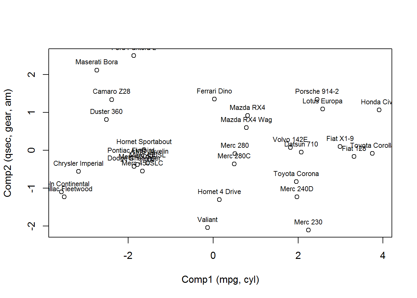
3 Closing word
Principal component analysis (PCA) and factor analysis factor analysis are similar because they both simplify the structure of a set of variables. However, there are some important differences between these two methods:
Principal component analysis starts with finding a low-dimensional linear subspace that best describes the data. Since the subspace is linear, it can be described by a linear model. It is therefore a descriptive explorative process. The factor analysis uses a linear model and tries to approximate the observed covariance or correlation matrix. It is therefore a model-based process.
In principal component analysis, there is a clear ranking of the vectors, given by the descending eigenvalues of the covariance or correlation matrix. In the factor analysis, the dimension of the factor space is first defined and all vectors stand side by side with equal rights.
In principal component analysis, a p-dimensional random vector x is represented by a linear combination of random vectors chosen so that the first addend explains as much of the variance of x as possible, the second addend as much as possible of the remaining variance, and so on. The principal component analysis is intended to explain the total variance of the variables as completely as possible. The aim of the factor analysis is to determine the covariances or correlations between the variables.
Principal component analysis is used to reduce the data to a smaller number of components. Factor analysis is used to determine the constructs underlying the data.
Source
Burger, S. V. (2018). Introduction to Machine Learning with R: Rigorous Mathematical Analysis. " O’Reilly Media, Inc.“.