library(tidyverse)
library(rpart)
library(caret)
library(randomForest)
library(party)
cu_summary <- read_csv("cu.summary.csv")Table of Content
- 1 Introduction
- 2 A simple tree model
- 2.1 Tree entropy and information gain
- 2.2 Visualize a simple tree model
- 3 Prune tree
- 4 Decision trees for regression
- 5 Decision trees for classification
- 6 Conditional inference trees
- 7 Closing word
1 Introduction
Decision trees are ordered, directed trees that serve to represent decision rules. The graphical representation as a tree diagram illustrates hierarchically successive decisions. Decision trees are an important part of information processing. They are often used not only in the field of data mining to derive strategies for route guidance, but also in machine learning. The process helps us in decision-making, as it visualizes different possibilities and scenarios.
For this post the dataset cu.summary from the package “rpart” was used. A copy of the record is available at https://drive.google.com/open?id=1o8rinf_SUZzsfAc_K7nI6Z7uhYyy_bZi.
2 A simple tree model
Let’s create an own decision tree as a fitting example.
a <- c("cloudy", "rainy", "sunny", "cloudy", "cloudy", "rainy", "rainy", "cloudy", "sunny", "sunny", "rainy", "sunny", "sunny")
b <- c("low", "low", "high", "high", "low", "high", "high", "high", "low", "low", "low", "low", "high")
c <- c("high", "normal", "normal", "high", "normal", "high", "normal", "normal", "high", "normal", "normal", "high", "high")
d <- c("yes", "yes", "yes", "yes", "yes", "no", "no", "yes", "no", "yes", "yes", "no", "no")
df <- data.frame(a, b, c, d)
colnames(df) <- c("Sky.Condition", "Wind.Speed", "Humidity", "Result")
df
## Sky.Condition Wind.Speed Humidity Result
## 1 cloudy low high yes
## 2 rainy low normal yes
## 3 sunny high normal yes
## 4 cloudy high high yes
## 5 cloudy low normal yes
## 6 rainy high high no
## 7 rainy high normal no
## 8 cloudy high normal yes
## 9 sunny low high no
## 10 sunny low normal yes
## 11 rainy low normal yes
## 12 sunny low high no
## 13 sunny high high no2.1 Tree entropy and information gain
Definition of entropy: Entropy is the measures of impurity, disorder or uncertainty in a bunch of examples.
Entropy controls how a Decision Tree decides to split the data. It actually effects how a Decision Tree draws its boundaries.
Definition of information gain: Information gain measures how much “information” a feature gives us about the class.
Why it matter ?
- Information gain is the main key that is used by Decision Tree Algorithms to construct a Decision Tree.
- Decision Trees algorithm will always tries to maximize Information gain.
- An attribute with highest Information gain will tested/split first.
Within R you can use the VarImpPlot() function to get a quick glance to see how to split the tree from the top down.
fit <- randomForest(factor(Result) ~ ., data = df)
varImpPlot(fit)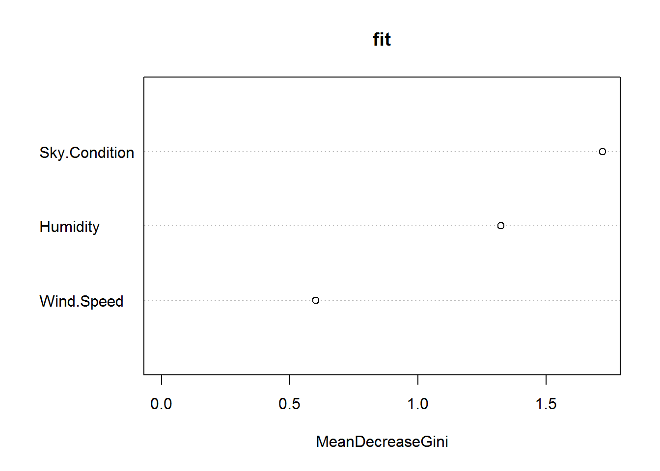
2.2 Visualize a simple tree model
fit2 <- rpart(Result~Sky.Condition + Wind.Speed + Humidity, method = "anova", data = df,
              control =rpart.control(minsplit =1,minbucket=1, cp=0))


plot(fit2, uniform = TRUE, margin=0.1)
text(fit2, use.n = TRUE, all=TRUE, cex=.8)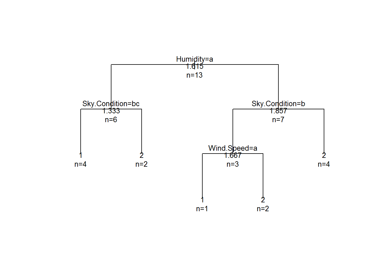
3 Prune tree
Overfitting is a general problem with decision trees. One solution is to prune the decision tree accordingly. Let’s look at the record we want to use for this example.
glimpse(cu_summary)## Observations: 117
## Variables: 6
## $ X1 <chr> "Acura Integra 4", "Dodge Colt 4", "Dodge Omni 4",...
## $ Price <int> 11950, 6851, 6995, 8895, 7402, 6319, 6695, 10125, ...
## $ Country <chr> "Japan", "Japan", "USA", "USA", "USA", "Korea", "J...
## $ Reliability <chr> "Much better", NA, "Much worse", "better", "worse"...
## $ Mileage <int> NA, NA, NA, 33, 33, 37, NA, NA, 32, NA, 32, 26, NA...
## $ Type <chr> "Small", "Small", "Small", "Small", "Small", "Smal...In this case we want to model a vehicle’s fuel efficiency, as given by the Mileage variable. Since Mileage is a numerical variable, it becomes a regression model as a result.
fit3 <- rpart(Mileage~Price + Reliability + Type + Country, method = "anova", data = cu_summary)

plot(fit3, uniform = TRUE, margin=0.1)
text(fit3, use.n = TRUE, all=TRUE, cex=.8)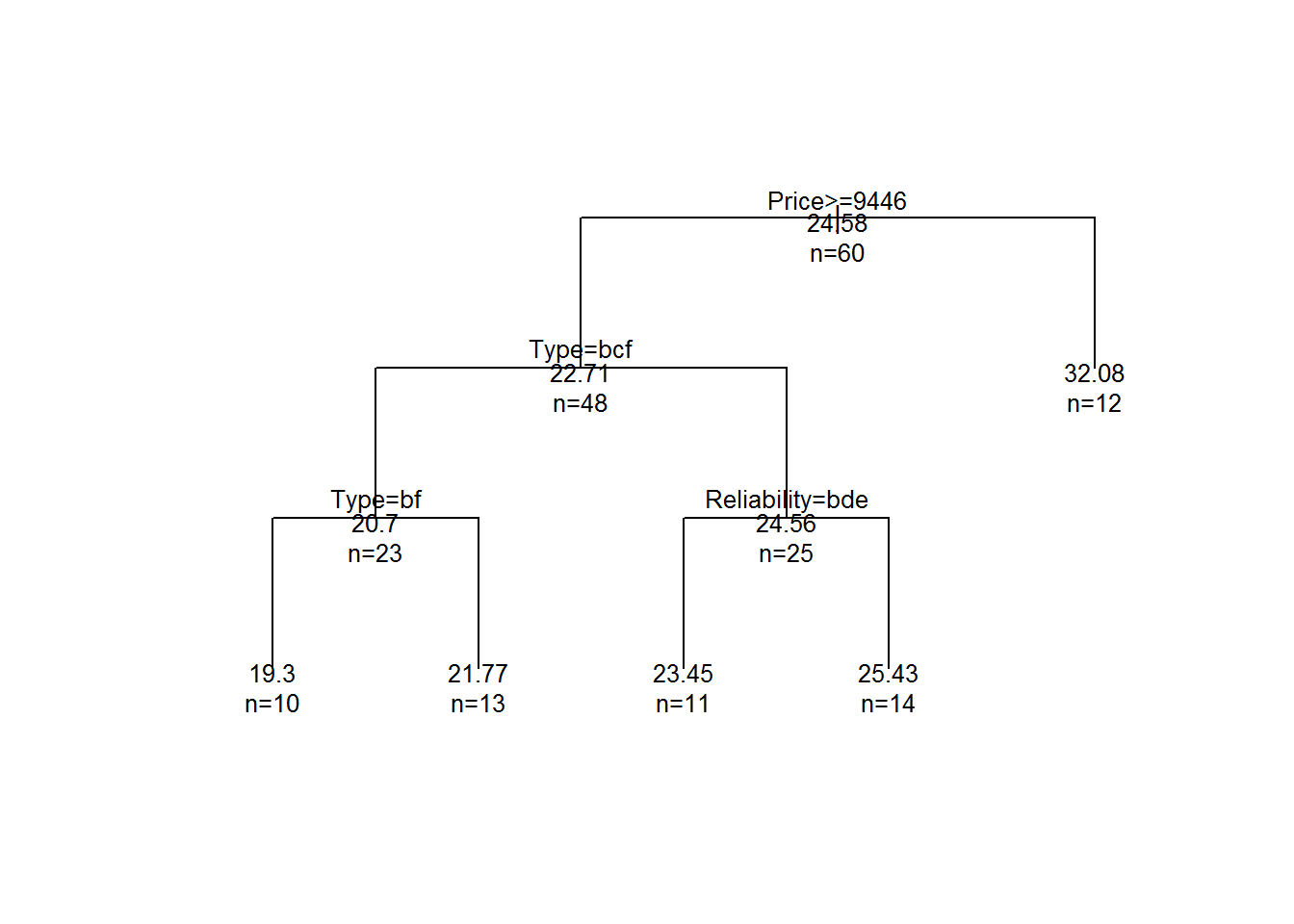
A precise way of knowing which parts to prune is to look at a tree’s complexity paramete, often refered to as the “CP”, which you can request with the plotcp function.
plotcp(fit3)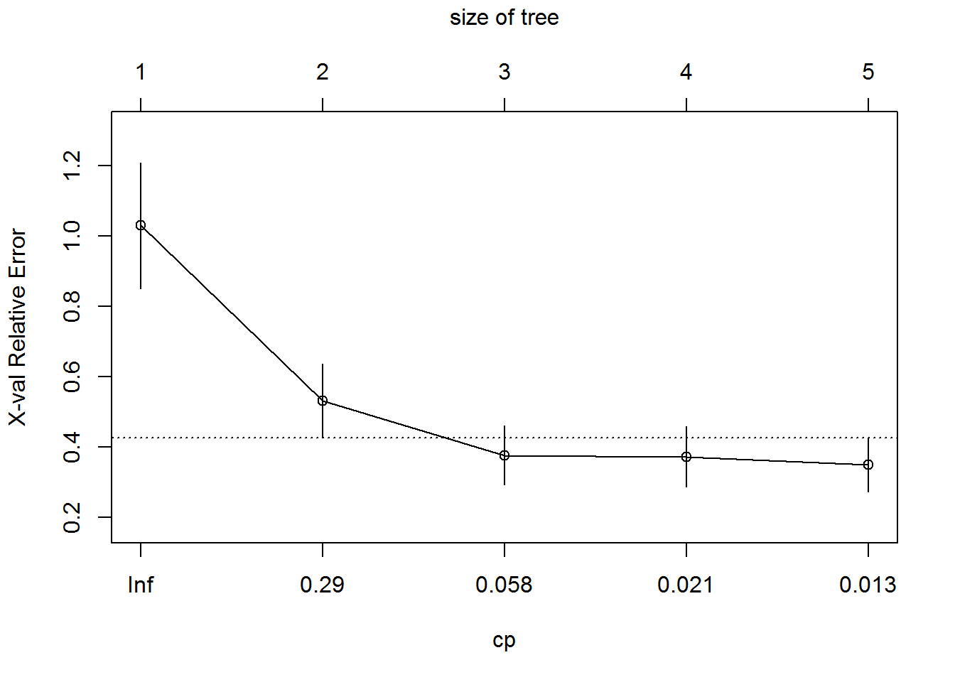
The complexy parameter is the amount by which splitting that tree node will improve the relative error.In the figure above, splitting it once improve the error by 0.29, and then less so for each additional split. You can see from the plot that the relative error is minimized at a tree size of 3 and the complexity paramter is below the dotted line threshold.
You can extract all these values programmatically from the model’s cptable, as follows:
fit3$cptable## CP nsplit rel error xerror xstd
## 1 0.62288527 0 1.0000000 1.0295681 0.17828009
## 2 0.13206061 1 0.3771147 0.5311535 0.10538275
## 3 0.02544094 2 0.2450541 0.3769875 0.08448195
## 4 0.01772069 3 0.2196132 0.3727303 0.08512904
## 5 0.01000000 4 0.2018925 0.3498613 0.07613958You can see that the error is minimized at tree size 3. Now let’s prune the previously created tree.
fit3.pruned <- prune(fit3, cp = fit3$cptable[which.min(fit3$cptable[,"xerror"]), "CP"])par(mfrow = c(1, 2))
plot(fit3, uniform = TRUE, margin=0.1, main = "Original decision tree")
text(fit3, use.n = TRUE, all=TRUE, cex=.8)
plot(fit3.pruned, uniform = TRUE, margin=0.1, main = "Pruned decision tree")
text(fit3.pruned, use.n = TRUE, all=TRUE, cex=.8)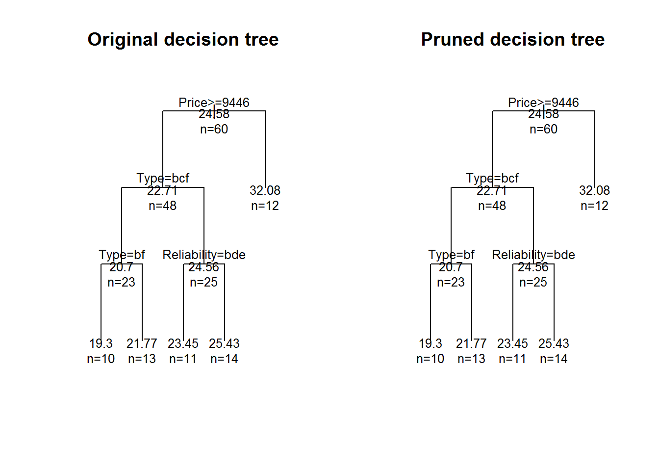
This example takes the complexity parameter and passes it to the prune() function to effectively eliminate any splits that don’t make the model reduce its error.
4 Decision trees for regression
cu.summary.compl <-  cu_summary[complete.cases(cu_summary), ]
nrow(cu.summary.compl)

data.samples <- sample(1:nrow(cu.summary.compl), nrow(cu.summary.compl)* 0.7, replace = FALSE)

training.data1 <- cu.summary.compl[data.samples, ]
test.data1 <- cu.summary.compl[-data.samples, ]

fit4 <- rpart(Mileage~Price + Reliability + Type + Country, method = "anova", data = training.data1)

fit4.pruned <- prune(fit4, cp = fit4$cptable[which.min(fit4$cptable[,"xerror"]), "CP"])

fit4.prediction <- predict(fit4.pruned, test.data1)

fit4.output <- data.frame(test.data1$Mileage, fit4.prediction)

fit4.RMSE <- sqrt(sum((fit4.output$test.data1.Mileage -fit4.output$fit4.prediction)^2)
                  /nrow(fit4.output))

fit4.RMSE
5 Decision trees for classification
cu.summary.compl <- cu_summary[complete.cases(cu_summary), ]

data.samples <- sample(1:nrow(cu.summary.compl), nrow(cu.summary.compl)* 0.7, replace = FALSE)

training.data2 <- cu.summary.compl[data.samples, ]
test.data2 <- cu.summary.compl[-data.samples, ]

fit5 <- rpart(Type~Price + Reliability + Mileage + Country, method = "class", data = training.data2)

fit5.pruned <- prune(fit5, cp = fit5$cptable[which.min(fit5$cptable[,"xerror"]), "CP"])

fit5.prediction <- predict(fit5.pruned, test.data2, type = "class")

table(fit5.prediction, test.data2$Type)
6 Conditional inference trees
Conditional inference trees estimate a regression relationship by binary recursive partitioning in a conditional inference framework.
cu.summary.new <- cu_summary[ ,2:6]Here’s an example of a conditional inference tree regression
fit6 <- ctree(Mileage ~ Price + factor(Reliability) + factor(Type) + factor(Country), data = na.omit(cu.summary.new))
plot(fit6)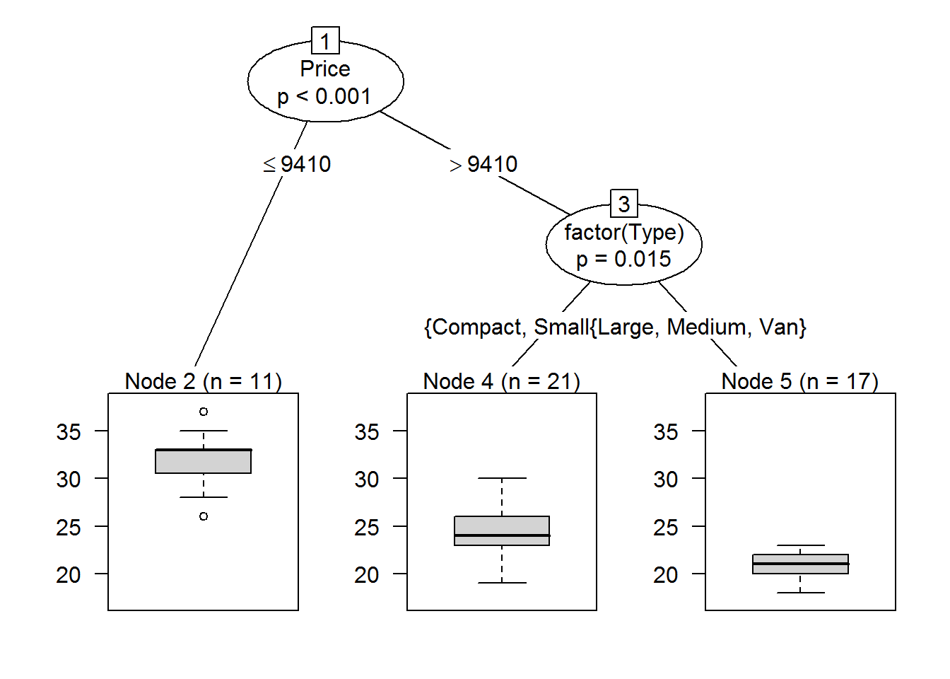
And here an other example of a conditional inference tree classification
fit7 <- ctree(factor(Type) ~ Price + factor(Reliability) + Mileage + factor(Country), data = na.omit(cu.summary.new))
plot(fit7)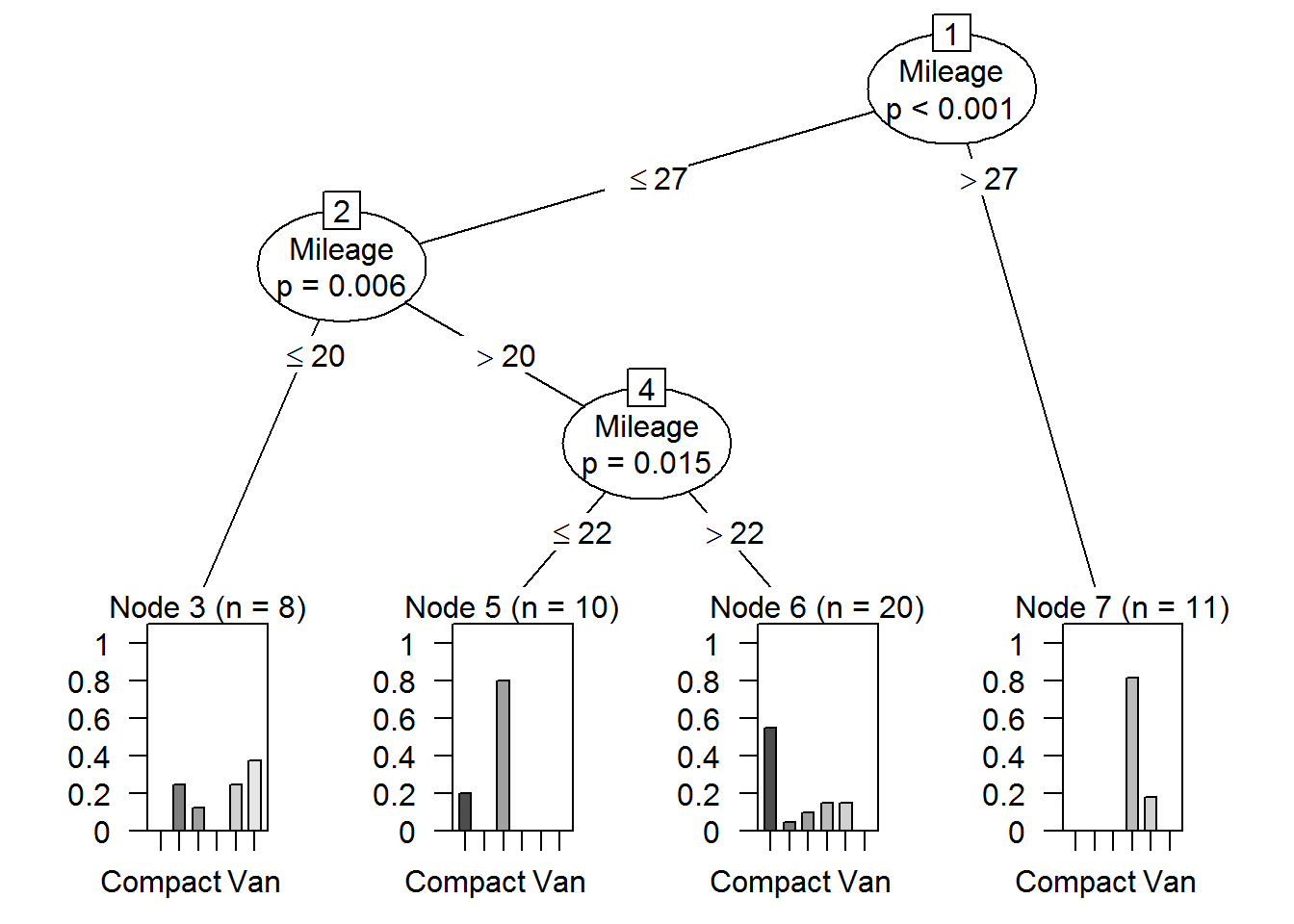
7 Closing word
Advantages and disadvantages of decision trees:
Due to their structure, decision trees are easy to understand, interpret and visualize. In doing so, a variable check or feature selection is implicitly performed. Both numerical and non-numerical data can be processed simultaneously relatively little effort on the part of the user for the data preparation requires.
On the other hand, too complex trees can be created that do not generalize the data well. This is called over-fitting. Small variations in the data can also make the trees unstable, creating a tree that does not solve the problem. This phenomenon is called variance.
Source
Burger, S. V. (2018). Introduction to Machine Learning with R: Rigorous Mathematical Analysis. " O’Reilly Media, Inc.“.