Table of Content

• 1 Introduction
• 2 Creation of two dependent variables
• 3 Train and test the simple regression model
• 4 Train and test the polynomial regression model
• 5 Train and test the exponential regression model
• 6 Conclusion

1 Introduction

This post deals with the subject of machine learning. In particular, the training and testing of data for a regression analysis will be considered.

2 Creation of two dependent variables

In the first step, two interdependent variables are generated.

set.seed(123)
x <- rnorm(100, 2, 1)
y <- exp(x) + rnorm(7, 0, 1)

## Warning in exp(x) + rnorm(7, 0, 1): Länge des längeren Objektes
##       ist kein Vielfaches der Länge des kürzeren Objektes

linear <- lm(y  ~ x)

plot(x, y)
abline(a = coef(linear[1], b = coef(linear[2], lty = 2)))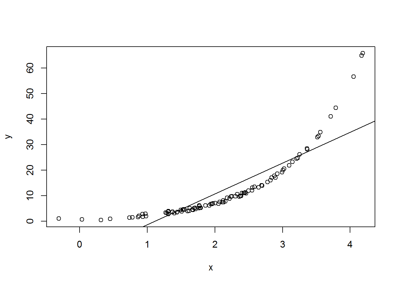

summary(linear)

## 
## Call:
## lm(formula = y ~ x)
## 
## Residuals:
##    Min     1Q Median     3Q    Max 
## -5.457 -4.115 -2.108  1.310 28.695 
## 
## Coefficients:
##             Estimate Std. Error t value Pr(>|t|)    
## (Intercept) -13.4079     1.6402  -8.175 1.07e-12 ***
## x            12.0637     0.7196  16.764  < 2e-16 ***
## ---
## Signif. codes:  0 '***' 0.001 '**' 0.01 '*' 0.05 '.' 0.1 ' ' 1
## 
## Residual standard error: 6.536 on 98 degrees of freedom
## Multiple R-squared:  0.7414, Adjusted R-squared:  0.7388 
## F-statistic:   281 on 1 and 98 DF,  p-value: < 2.2e-16

3 Train and test the simple regression model

Subsequently, the newly created data set is divided into a training part (80%) and a test part (20%).

data <- data.frame(x, y)
data.samples <- sample(1:nrow(data), nrow(data) * 0.8, replace = FALSE)
training.data <- data[data.samples, ]
test.data <- data[-data.samples, ]

Now the regression model can be traniniert with the training data.

train.linear <- lm(y ~ x, training.data)
train.output <- predict(train.linear, test.data)

The quality of the prediction can be determined using the root mean square error (RMSE).

\[RMSE = \sqrt{\frac{1}{n}\Sigma_{i=1}^{n}{\Big(\frac{d_i -f_i}{\sigma_i}\Big)^2}}\]

RMSE.df <- data.frame(predicted = train.output, actual = test.data$y, 
                      SE = ((train.output - test.data$y)^2/length(train.output)))

head(RMSE.df)

##    predicted    actual           SE
## 6  29.249080 41.016228 6.923288e+00
## 9   2.895065  3.974740 5.828484e-02
## 11 23.861977 24.782946 4.240916e-02
## 15  4.332535  3.527879 3.237358e-02
## 20  5.243763  4.560276 2.335772e-02
## 25  3.573288  3.607379 5.810787e-05

sqrt(sum(RMSE.df$SE))

## [1] 8.065677

We get a RMSE value of 8.07. To see how good this value is, it can be compared to other RMSE values.

4 Train and test the polynomial regression model

train.polyn <- lm(y ~ poly(x, 4), training.data)
polyn.output <- predict(train.polyn, test.data)

RMSE.polyn.df <- data.frame(predicted = polyn.output, actual = test.data$y, 
                                  SE = ((polyn.output - test.data$y)^2/length(polyn.output)))

head(RMSE.polyn.df)

##    predicted    actual           SE
## 6  41.203433 41.016228 1.752296e-03
## 9   3.333099  3.974740 2.058515e-02
## 11 24.954389 24.782946 1.469629e-03
## 15  3.873118  3.527879 5.959505e-03
## 20  4.245259  4.560276 4.961783e-03
## 25  3.581171  3.607379 3.434285e-05

sqrt(sum(RMSE.polyn.df$SE))

## [1] 0.4690057

With a RMSE value of 0.47, we can see that the quality of the prediction has already improved significantly.

5 Train and test the exponential regression model

train.exponential <- lm(y ~ exp(x) + x, training.data)
exponential.output <- predict(train.exponential, test.data)

RMSE.exponential.df <- data.frame(predicted = exponential.output, actual = test.data$y, 
                                  SE = ((exponential.output - test.data$y)^2/length(exponential.output)))

head(RMSE.exponential.df)

##    predicted    actual           SE
## 6  40.807386 41.016228 2.180737e-03
## 9   3.291509  3.974740 2.334023e-02
## 11 24.788044 24.782946 1.299666e-06
## 15  3.811601  3.527879 4.024919e-03
## 20  4.178644  4.560276 7.282133e-03
## 25  3.528361  3.607379 3.121932e-04

sqrt(sum(RMSE.exponential.df$SE))

## [1] 0.3703497

An even better predictive value we get in this case with the exponential regression model. RMSE = 0.37

6 Conclusion

This should be a brief demonstration of how regression models can be trained and their predictive power improved.

Source

Burger, S. V. (2018). Introduction to Machine Learning with R: Rigorous Mathematical Analysis. " O’Reilly Media, Inc.“.