Table of Content

• 1 Introduction
• 2 What is Web Scraping?
• 3 Annotation
• 4 The web scraping process
• 5 A few graphic analysis
• 6 A brief insight of text mining
• 7 Conclusion

1 Introduction

The amount of data and information available on the Internet is growing exponentially. The amount of data available on the Web opens up new possibilities for a data scientist, such as web scraping. In today’s world, all the data we need is already available on the Internet. The only thing that prevents some people from using them is accessing them. With the help of this post, this barrier can be overcome.

2 What is Web Scraping?

Web scraping is a technique for converting the data present in unstructured format (HTML tags) over the web to the structured format which can easily be accessed and used. In this post, the most popular feature films of the year 2018 will be removed from the “IMDb” website.

3 Annotation

For users who are not very familiar with HTML and CSS, I recommend using the open source software called Selector Gadget, which is more than enough for anyone to do web scraping. You can download the Selector Gadget extension “here”.

4 The web scraping process

url <- "http://www.imdb.com/search/title?count=100&release_date=2016,2016&title_type=feature"
webpage <- read_html(url)


rank_data_html <- html_nodes(webpage,'.text-primary')
rank_data <- html_text(rank_data_html)
rank_data<-as.numeric(rank_data)

title_data_html <- html_nodes(webpage,'.lister-item-header a')
title_data <- html_text(title_data_html)

description_data_html <- html_nodes(webpage,'.ratings-bar+ .text-muted')
description_data <- html_text(description_data_html)
description_data<-gsub("\n","",description_data)

runtime_data_html <- html_nodes(webpage,'.text-muted .runtime')
runtime_data <- html_text(runtime_data_html)
runtime_data<-gsub(" min","",runtime_data)
runtime_data<-as.numeric(runtime_data)

genre_data_html <- html_nodes(webpage,'.genre')
genre_data <- html_text(genre_data_html)
genre_data<-gsub("\n","",genre_data)
genre_data<-gsub(" ","",genre_data)
genre_data<-gsub(",.*","",genre_data)
genre_data<-as.factor(genre_data)

rating_data_html <- html_nodes(webpage,'.ratings-imdb-rating strong')
rating_data <- html_text(rating_data_html)
rating_data<-as.numeric(rating_data)

votes_data_html <- html_nodes(webpage,'.sort-num_votes-visible span:nth-child(2)')
votes_data <- html_text(votes_data_html)
votes_data<-gsub(",","",votes_data)
votes_data<-as.numeric(votes_data)

directors_data_html <- html_nodes(webpage,'.text-muted+ p a:nth-child(1)')
directors_data <- html_text(directors_data_html)
directors_data<-as.factor(directors_data)

actors_data_html <- html_nodes(webpage,'.lister-item-content .ghost+ a')
actors_data <- html_text(actors_data_html)
actors_data<-as.factor(actors_data)




movies_df<-data.frame(Rank = rank_data, Title = title_data,
                      
                      Description = description_data, Runtime = runtime_data,
                      
                      Genre = genre_data, Rating = rating_data,
                      
                      Votes = votes_data, Director = directors_data, Actor = actors_data)



glimpse(movies_df)

## Observations: 100
## Variables: 9
## $ Rank        <dbl> 1, 2, 3, 4, 5, 6, 7, 8, 9, 10, 11, 12, 13, 14, 15,...
## $ Title       <fct> Phantastische Tierwesen und wo sie zu finden sind,...
## $ Description <fct>     The adventures of writer Newt Scamander in New...
## $ Runtime     <dbl> 133, 106, 123, 117, 108, 116, 147, 133, 105, 116, ...
## $ Genre       <fct> Adventure, Adventure, Action, Horror, Action, Dram...
## $ Rating      <dbl> 7.3, 7.4, 6.1, 7.3, 8.0, 7.0, 7.8, 7.8, 5.8, 7.9, ...
## $ Votes       <dbl> 338250, 233381, 505590, 298641, 780515, 293013, 53...
## $ Director    <fct> David Yates, Jon Favreau, David Ayer, M. Night Shy...
## $ Actor       <fct> Eddie Redmayne, Neel Sethi, Will Smith, James McAv...

5 A few graphic analysis

Now we are able to analyze the pulled data. Below are some examples:

qplot(data = movies_df,Runtime,fill = Genre, bins = 30)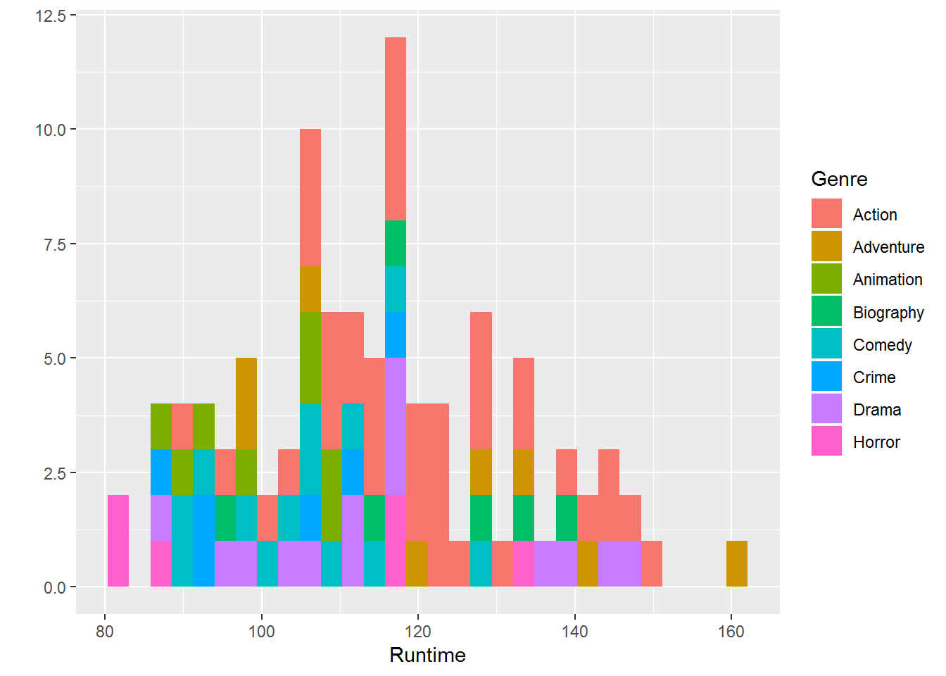

ggplot(movies_df,aes(x=Runtime,y=Rating))+
  geom_point(aes(size=Votes,col=Genre))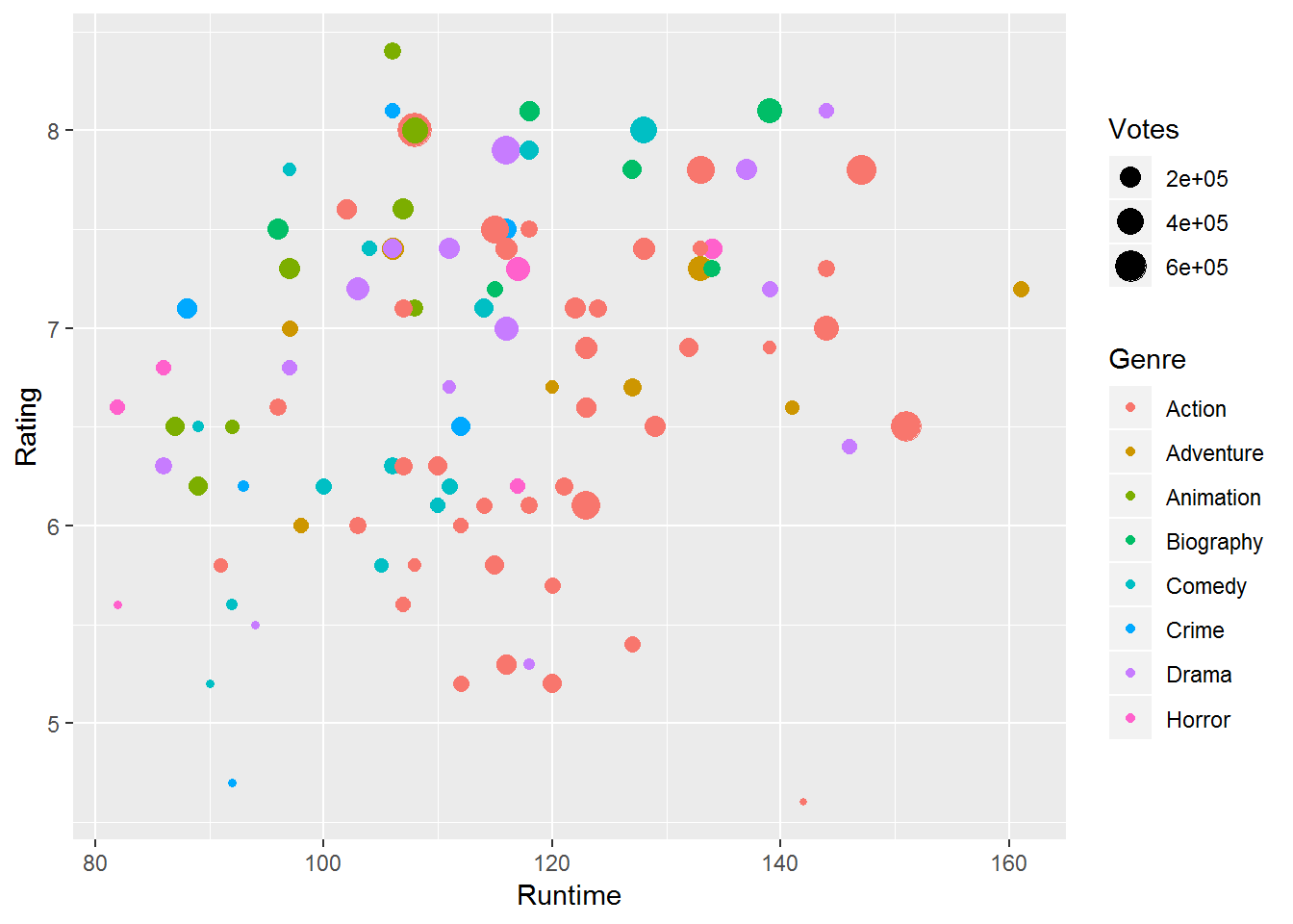

ggplot(movies_df,aes(x=Runtime,y=Votes))+
  geom_point(aes(size=Rating,col=Genre))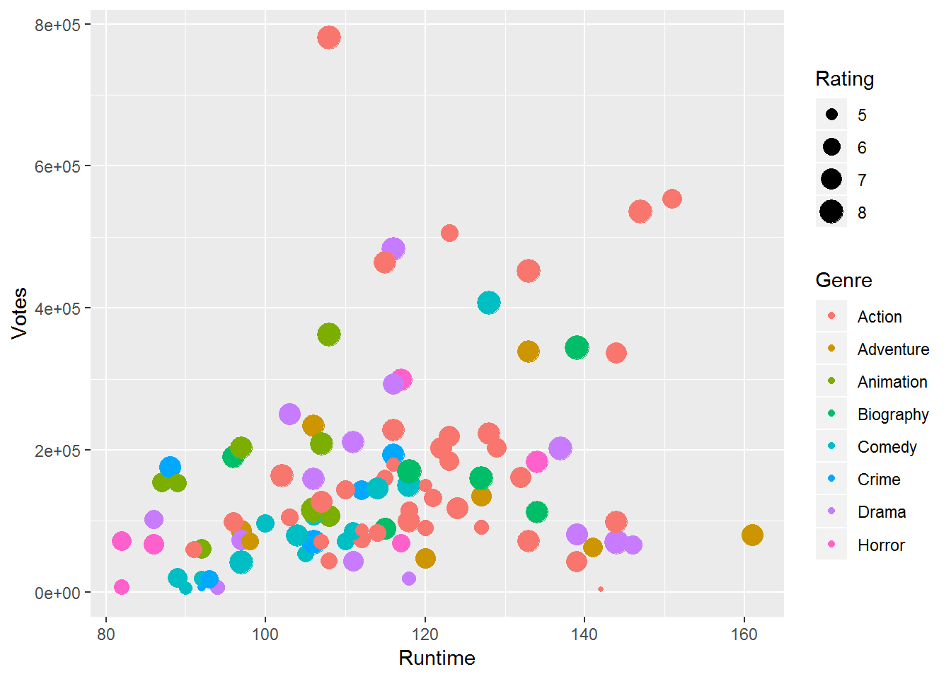

movies_df_2 <- movies_df %>% count(Genre)
ggplot(movies_df_2, aes(x=Genre, y=n)) +
  geom_bar(stat="identity", width=0.5) + coord_flip()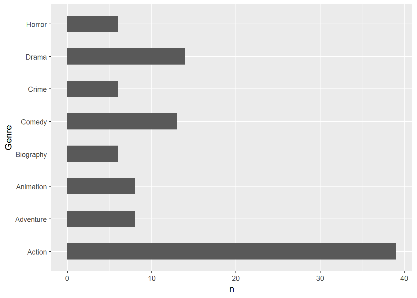

6 A brief insight of text mining

I am interested in the words used within the movie description.

movies_df$Description <- as.character(movies_df$Description)
text <- movies_df %>% select(Description)
tidy_text <- text %>% unnest_tokens(word, Description)
tidy_text %>% count(word, sort = TRUE)

## # A tibble: 1,254 x 2
##    word      n
##    <chr> <int>
##  1 a       163
##  2 the     161
##  3 to       91
##  4 of       89
##  5 in       66
##  6 and      58
##  7 his      31
##  8 with     28
##  9 is       26
## 10 an       25
## # ... with 1,244 more rows

Ok, we see some unwanted stop words… Let’s fix this:

data("stop_words")

tidy_text <- tidy_text %>% anti_join(stop_words)

## Joining, by = "word"

tidy_text %>% count(word, sort = TRUE)

## # A tibble: 1,056 x 2
##    word         n
##    <chr>    <int>
##  1 world       12
##  2 life        10
##  3 american     7
##  4 father       7
##  5 journey      7
##  6 city         6
##  7 save         6
##  8 story        6
##  9 death        5
## 10 home         5
## # ... with 1,046 more rows

We can also visualize this

tidy_text %>% count(word, sort = TRUE) %>% filter(n > 4) %>% mutate(word = reorder(word, n)) %>%
  ggplot(aes(word, n)) +
  geom_col() +
  xlab(NULL) +
  coord_flip()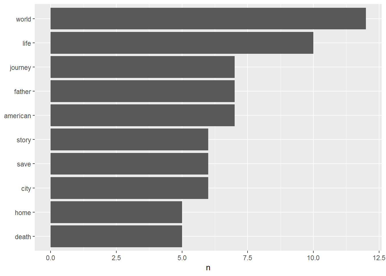

tidy_text %>% anti_join(stop_words) %>% count(word) %>% with(wordcloud(word, n, max.words = 100))

## Joining, by = "word"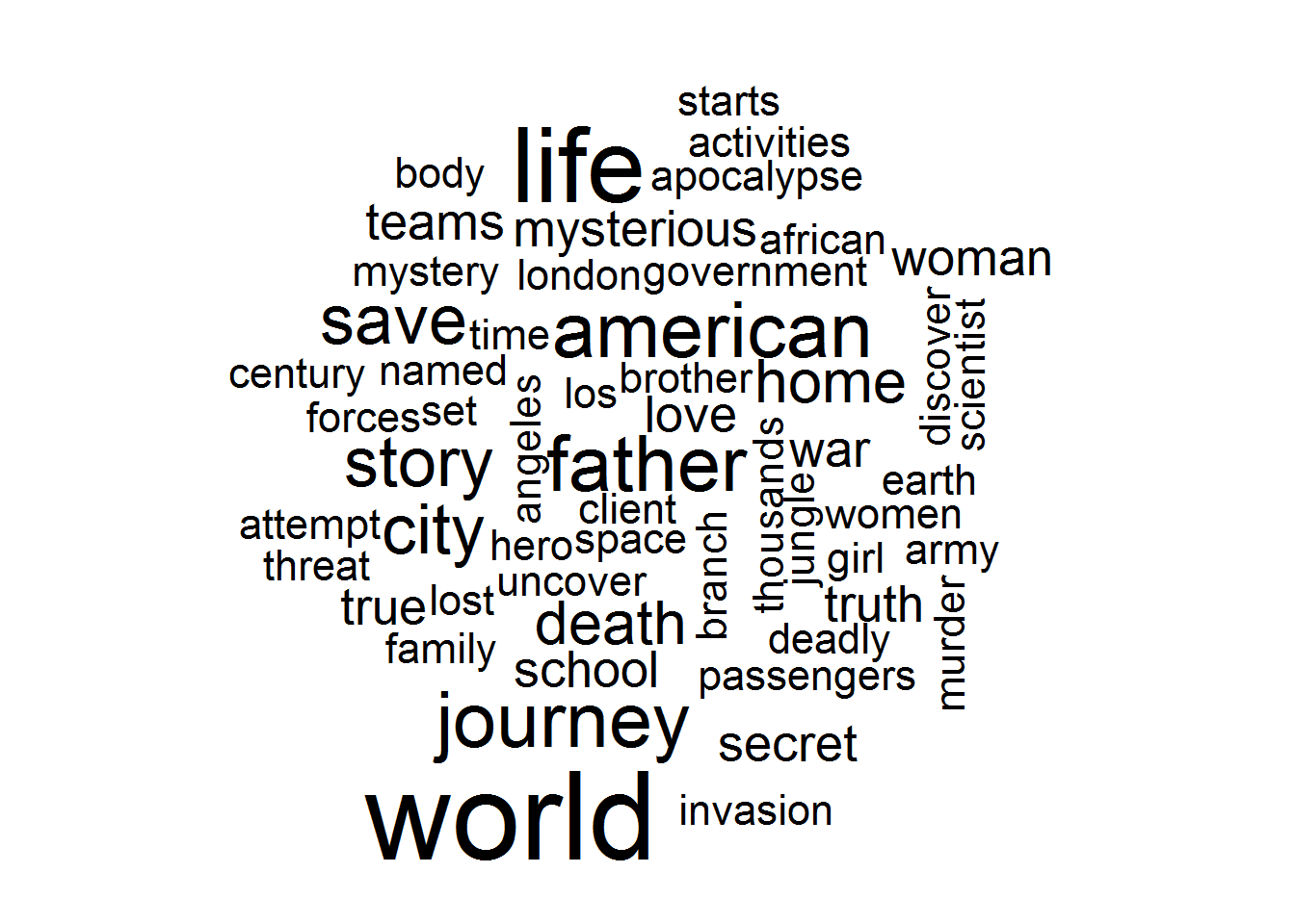

7 Conclusion

One might wonder, what you actually web scraping need for. The answer es as short as simple: the possibilities with web scraping are almost unlimited.